
Figure 3.
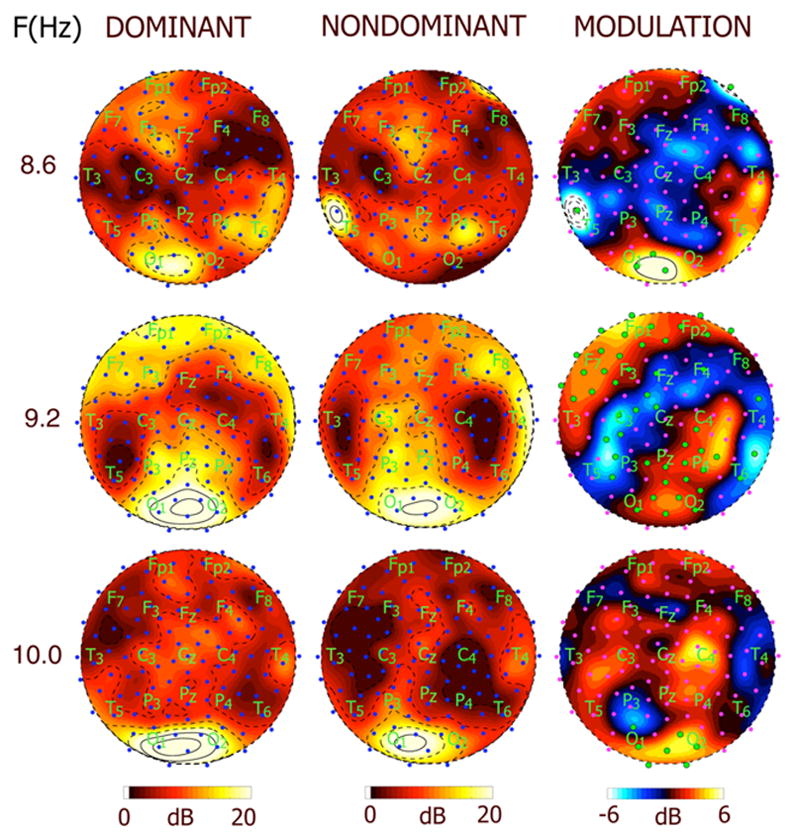
Topographic maps of SNR and power modulation (M) at three different stimulus frequencies for subject RY. Each row corresponds to a different stimulus frequency (A) 8.6 Hz (B) 9.2 Hz (C) 10 Hz. The column on the left shows map of SNR at the three frequencies during perceptual dominance (perceiving the stimulus). The column in the middle shows maps of SNR during perceptual nondominance (perceiving a rival stimulus presented at a different frequency). Contour lines are at intervals of 3.3 dB, with solid contour lines at and above 20 dB and dashed lines below 20 dB. The column on the right shows maps of power modulation M in dB. Contour intervals are at 1 dB with solid contour lines at and above 6 dB and dashed contour lines at and below −6 dB. Note that the distribution and modulation of the response is similar at adjacent frequencies, but can be recorded more easily at the global resonance frequency.