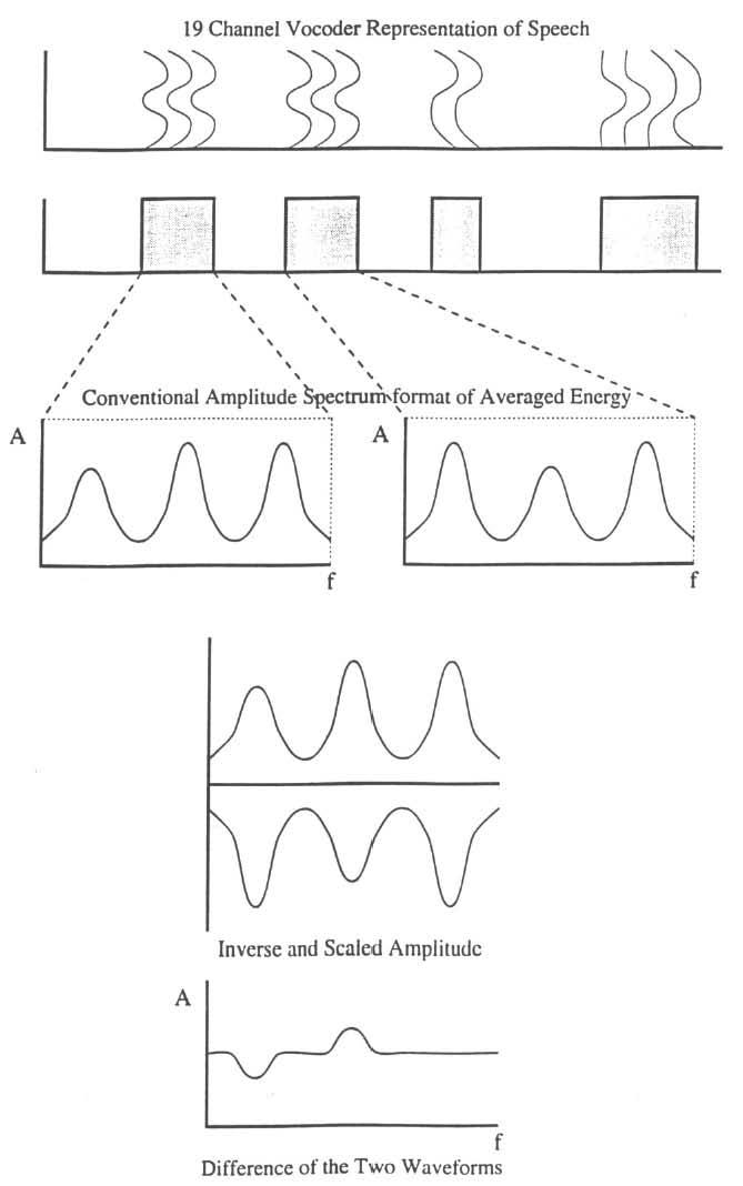
Figure 4.

Schematic summary of the steps involved in computing spectral measures between ATE sections for a repetition. The spectra in successive 10 ms frames are shown at the top: Time is along the abscissa, frequency along the ordinate, and the solid line indicates relative energy. The location of ATE (shaded) and BTE (white) regions (obtained in the way summarized in Figure 3) are indicated in the section beneath. The averaged spectra for the first and second ATE regions are depicted on the left and right of the third panel in standard amplitude spectrum-format. The amplitude spectrum of the first ATE region and the scaled and inverted second spectrum are next shown on the same axes. The differenced waveforms are shown in the final section. The SD across all 19 spectral coefficients is taken. The steps involved in computing spectral measures between BTE sections and across adjacent ATE and BTE sections is similar.
