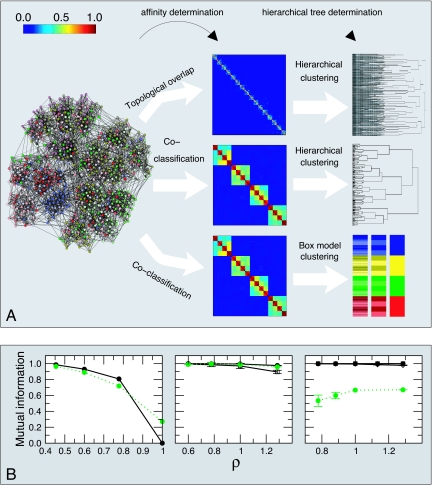
Fig. 2.
Affinity measures and clustering methods. (A) We generate a model network comprised of 640 nodes with average degree 16 and with a three-level hierarchical structure (see SI Fig. 8 for results for a network with a “flat” organization of the nodes). We show the affinity matrices Aij obtained for two different measures: (i) topological overlap (11) and (ii) coclassification (see text and Supplementary Information). The color scale goes from red for an affinity of one to dark blue for an affinity of zero. At the far right, we show the hierarchical tree obtained by using two different methods: hierarchical clustering and the “box clustering” method we propose. In the hierarchical clustering tree, the vertical axis shows the average distance, dij = 1 − Aij, of the matrix elements that have already merged. In the box-model clustering tree, each row corresponds to one hierarchical level. Different colors indicate different modules at that level. To better identify which are the submodules at a lower level, we color the nodes in the submodules with shades of the color used for the modules in the level above. Note that topological overlap fails to find any modular structure beyond a locally dense connectivity pattern. In contrast, the coclassification measure clearly reveals the hierarchical organization of the network by the “nested-box” pattern along the diagonal. Significantly, the hierarchical tree obtained via hierarchical clustering fails to reproduce the clear three-level hierarchical structure that the affinity matrix displays, whereas the box-model clustering tree accurately reproduces the three-level hierarchical organization of the network. (B) Accuracy of the method. We generate networks with 640 nodes and with built-in hierarchical structure comprising one (Left), two (Center), and three (Right) levels. The top level always comprises four modules of 160 nodes each. For networks with a second level, each of the top-level modules is organized into four submodules of 40 nodes. For the networks with three levels, each level-two module is further split into four submodules of 10 nodes. We build networks with different degrees of level cohesiveness by tuning a single parameter ρ (see SI Text). For low values of ρ, the levels are very cohesive, for high values of ρ the levels are weakly cohesive. Because we know a priori which are the nodes that should be coclassified at each level, we measure the accuracy as the mutual information between the empirical partition of the nodes and the theoretical one (23). We plot the mutual information versus ρ and, for comparison, we also plot the accuracy of a standard community detection algorithm (24) in finding the top level of the networks (dashed green line). Each point is the average over 10 different realizations of the network. Filled circles, empty squares, and filled diamonds represent the accuracy at the top, middle, and lowest levels, respectively. Note that our method is as good at detecting communities as a standard community detection algorithm for networks with a flat organization of the nodes. Additionally, our method is able to detect the top level for all cases analyzed, whereas standard modularity optimization algorithms are not.

