Line spectral analysis for harmonizable processes

Abstract

Harmonizable processes with spectral mass concentrated on a number of straight lines are considered. The asymptotic behavior of the bias and covariance of a number of spectral estimates is described. The results generalize those obtained for periodic and almost periodic processes.

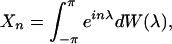
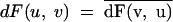
Let {X_t} be a continuous time parameter harmonizable process continuous in mean square, −∞ < t < ∞, with EX_t ≡ 0. By this we mean that the covariance function r(t, τ) = E(X_tτ) has a Fourier representation

1

with F(λ, μ) a function of bounded variation. This implies that X_t itself has a Fourier representation in mean square

2

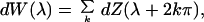
in terms of a random function Z(λ) with

3

If the process X_t is real-valued,

4

In the case of a weakly stationary process r(t, τ) = r(t − τ, 0) and all the spectral mass is located on the diagonal line λ = μ. If the process is periodic with

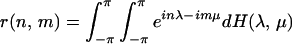
for some period a or almost periodic the spectral mass is located on a finite or countable number of lines in the (λ, μ) plane with slope one. If the process is discretely observed X_n, n = 0, ±1, ±2, … there is an analogous representation

5

with

6

The folding of F(λ, μ) to obtain H(λ, μ) is referred to as aliasing.

There is an enormous literature concerned with spectral estimation in the case of stationary processes (1). Recently efforts have been made to obtain analogous results on spectral estimation for periodic and almost periodic processes (2–7). It is well known that one generally does not have consistent estimates of spectral mass for a harmonizable process when the function F (or H) is absolutely continuous with a spectral density function f, dF(λ, μ) = f(λ, μ)dλdμ, with f(λ, μ) ≠ 0 on a set of positive two-dimensional Lebesgue measure, and one is sampling from the process X_−n, … , X_n and n → ∞. A simple example is given by X₀ normal with mean zero and variance one and X_k ≡ 0 with probability one for k ≠ 0. It is clear that consistency of spectral estimates in the case of stationary and periodic processes is due to the fact that the spectral mass is concentrated on lines that in these cases happen to be of slope one. We shall consider spectral estimation for harmonizable processes when the spectrum is concentrated on a finite (or possibly countable) number of lines. 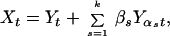For convenience the slope of the lines will be assumed to be positive, though the modification for negative slopes is clear. A simple example of a harmonizable process with spectral mass on lines is given by

7

where Y_t is stationary and β_s and α_s are real and positive numbers, respectively. The object is to give some insight into an interesting class of nonstationary processes.

Assume that X_t is a harmonizable real-valued process as already specified with

A1.  All its spectral mass on a finite number of lines with positive slope

A2.  The spectral mass on the line u = a_iv + b_i is given by a continuously differentiable spectral density f_ai,bi(v) if a_i ≤ 1. Notice that the real-valued property implies that if u = av + b is a line of spectral mass, then so are the lines u = av − b and u = a⁻¹v ± a⁻¹b. If there are lines of nonzero spectral mass, the diagonal λ = μ must be one of them with positive spectral mass. The condition

implies if u = av + b is a line of nonzero spectral mass, then so is u = a⁻¹(v − b) with

A3.  The spectral densities f_ai,bi(v) and their derivatives are bounded in absolute value by a function h(v) that is a monotonic decreasing function of |v| that decreases to zero as |v| → ∞ and that is integrable as a function of v.

As already remarked, aliasing or folding of the spectral mass occurs when the process is discretely sampled at times n = …  , − 1, 0, 1, … rather than continuously. The following simple remark indicates how a process with line spectra may differ from a stationary or almost periodic process in terms of aliasing. The aliasing in the case of a harmonizable process has a more complicated character.

Proposition 1. Let X_t be a continuous time parameter process continuous in mean square satisfying conditions A1–A3. Assume that the lines of spectral support have spectral density nonzero at all points v, |v| > s for some s > 0. The process discretely observed X_n then has a countably dense set of lines of support in [−π, π]² if and only if one of the lines of spectral support of X_t has irrational slope a.

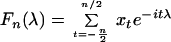
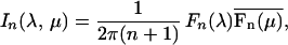
The Periodogram

We shall consider spectral estimation for the discretely observed process X_n. The estimates will be obtained by smoothing a version of the periodogram. Before dealing with the spectral estimates, approximations for the mean and covariances of the periodogram are obtained. Let

8

be the finite Fourier transform of the data x_−n/2, … , x_n/2. The periodogram

9

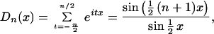
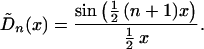
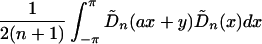
and it is to be understood that |λ|, |μ| ≤ π with −π identified with π so that in effect one is dealing with the torus in (λ, μ). Set

These expressions are versions of the Dirichlet kernel adapted to (−π, π] and (−∞, ∞). The following result is useful in obtaining the expressions for the mean and covariance of the periodogram.

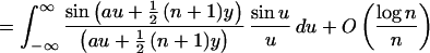
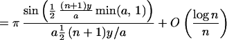
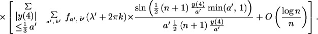
Lemma 1. If a > 0, |y| < π,

10

and

11

if |y| ≤ a/3, while if |y| ≥ a/3 the expression is itself of order log n/n.

Whenever we refer to an expression ω = z mod 2π it is understood that −π < ω ≤ π. Let {u} be the integer ℓ such that −1/2 < u − ℓ ≤ 1/2. Our version of z mod 2π is then z mod 2π = z − {z/(2π)}2π. In the following an approximation is given for EI_n(αμ + ω, μ) with the condition imposed that α > 0 and −π < αμ + ω, μ ≤ π. Let y = y(k, a, b) = (2πka + (a − α)μ + b − ω) mod 2π.

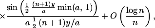
Theorem 1. The mean

12

where in the sum it is understood that the k are integers and the pairs (a, b) correspond to the lines u = av + b in the spectrum of the continuous time parameter process X_t that one is observing at integer t.

In the following result an approximation is given for the cov(I_n(αμ + ω, μ), I_n(α′μ′ + ω′, μ′)). Here

13

with λ = αμ + ω, λ′ = α′μ′ + ω′, −π < λ, λ′, μ, μ′ ≤ π. Also (a, b), (a′, b′) correspond to lines in the spectrum of the continuous time parameter process X_t that one is observing at integer times.

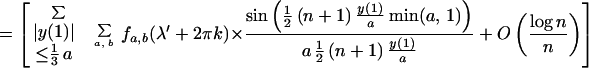
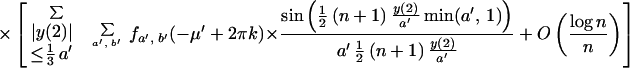
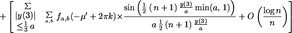
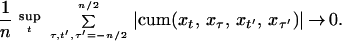
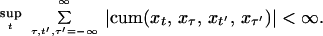
Theorem 2. The covariance in the case of a normal process X_t is

14

Corollary 1. The result of Theorem 2 holds with an additional error term O(1/n) for a nongaussian harmonizable process with finite fourth-order moments if the fourth-order cumulants satisfy

15

This will be the case if

16

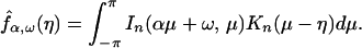
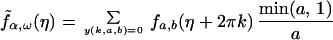
Spectral Estimates

We consider an estimate f̂_α,ω(η) of f̃_α,ω(η) obtained by smoothing the periodogram. Let K(η) be a nonnegative bounded weight function of finite support with ∫ K(η)dy = 1. The weight function K_n(η) = b_n⁻¹ K(b_n⁻¹η) with b_n ↓ 0 as n → ∞ and nb_n → ∞. The weight functions K_n should be considered as functions on the circle (−π, π] with −π identified with π. The estimate

17

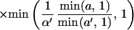
Proposition 2. If A2 is strengthened so that the spectral densities f_ai,bi(ν) are assumed to be twice continuously differentiable and K is symmetric, then

where

as n → ∞.

The asymptotic behavior of covariances is described in the following result.

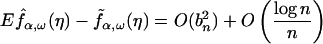
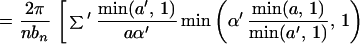
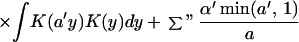
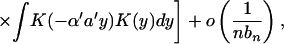
Theorem 3. Let X_t be a continuous time parameter harmonizable process continuous in mean square satisfying assumptions A1–A3 and 16. Then

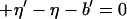
where the first sum Σ′ is over a, a′, b, b′, k, k′ such that

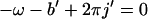
with 2πj′ = 2πk′a′ + b′ − ((2πk′a′ + b′)mod 2π), while the second sum Σ" is over a, a′, b, b′, k, k′ such that

with

In the almost periodic case we have the following corollary.

Corollary 2. If the assumptions of Theorem 3 are satisfied with X_t almost periodic

where the first sum is over b, b′, k, k′ such that

with 2πj′ = 2πk′ + b′ − ((b′)mod 2π) while the second sum is over b, b′, k, k′ with

with

On heuristic grounds one would expect to be able to estimate a spectral density localized on a piecewise smooth curve in the plane.