Figure 2.

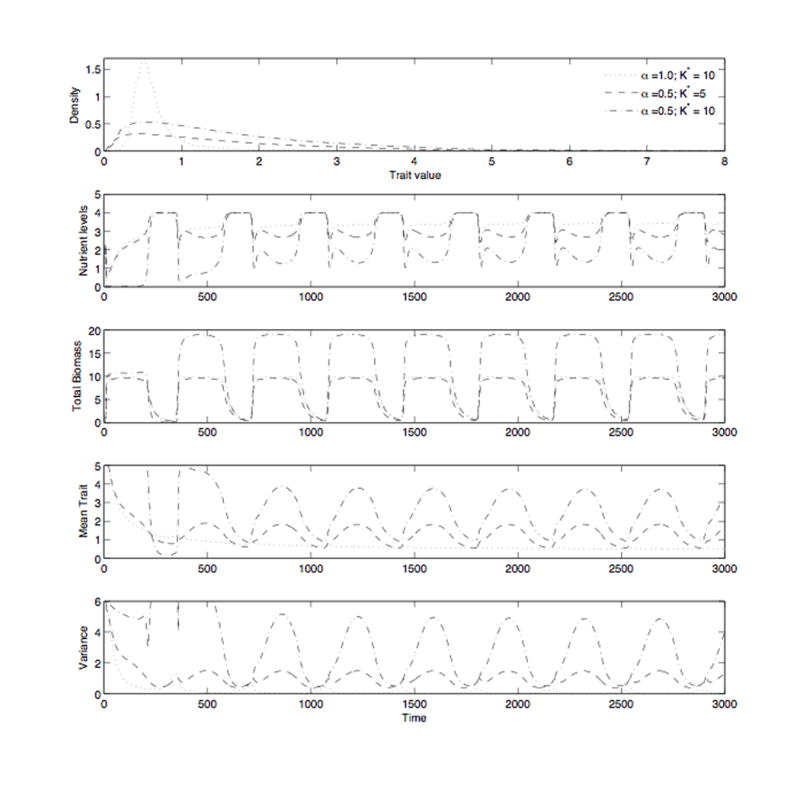
Simulation results for Eqs. (9-10) using the parameter values p = 1, m = 0.01, c = 0.02, inp = 0.2, d = 0.1, and a total immigration per time step of 0.001. The results are for three different simulations corresponding to α = 1 with a carrying capacity of K^* = 10 and to α = 0.5 with carrying capacities of K^* = 5 and K^* = 10. We use the notation K^* here, instead of K as in Sec. (4), to differentiate between the un-normalized (K) and normalized (K → αK) carrying capacities. For α = 1, K = αK, so K^* = 10 represents both cases. For α = 0.5, K^* = 10 is the un-normalized carrying capacity and K^* = α10 = 5 is the normalized value. The simulation with α set to 1 represents high competition/low complementarity and 0.5 represents low competition/high complementarity. For α = 0.5 the un-normalized value of the carrying capacity (K^* = 10) corresponds to over-yielding and larger total biomass (maximal biomass of 20), while the normalized value (K^* = 5) accounts for the effects of over-yielding and total biomass (maximal biomass of 10), revealing the effects of complementarity that are due solely to reduced competition. Panel 1 displays the trait distribution density as a function of the trait z, where values were averaged over the last cycle of the simulation. Panel 2 shows the dynamics of nutrients mainly as determined by seasonal changes in productivity. Panel 3 shows the total community biomass, C_T . Panel 4 depicts the mean trait for each community. Panel 5 displays the dynamics of the trait variance and shows that increased complementarity in resource use leads to greater trait variance.