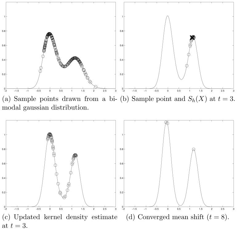
Fig. 1.

Graphical illustration of the mean shift algorithm where sample points were randomly drawn from a bi-modal mixture-of-gaussians distribution. In (a), the sample points are displayed on top of a kernel density estimate of the underlying distribution (see equation (1)). At each iteration of the mean shift, samples from the neighborhood S_h(X) are used to form the mean shift, M_h(X). This is shown in (b) for t = 3 and a sample point $x_i^3$ marked by an “X”, with the points in $S_h\left(x_i^3\right)$ marked by open circles. The algorithm converges rapidly, (d) shows the updated sample points converged to the modes of the underlying distribution at t = 8. In this case, we have updated the kernel density estimate at each iteration, resulting in a narrowing of the peaks in (d).