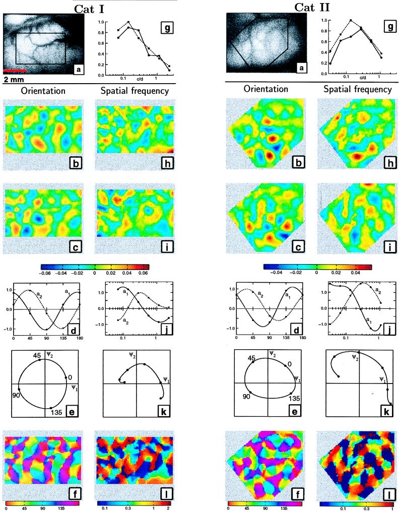
Figure 1.
(Left and Right) Data from two anesthetized cats. (a) Exposed visual cortex; the region used for detailed analysis is outlined. (b and c) The two “basis” pictures ψn(x) that generate the averaged orientation optical responses. (d) Weighting coefficient curves, an(θ), which weight basis pictures b and c to yield the orientation response at a given angle. (e) Locus of orientation optical response “vectors” in two-dimensional section through pixel space. (f) Pattern of orientation pinwheels; color indicates preferred angle in degrees. (g) Strength of “orthogonal orientation difference response” vs. spatial frequency; the two curves are vertical–horizontal (solid) and diagonal (dashed) differences. Logarithmic cycles-per-degree scale also appears in j below. (h and i) The two basis pictures ψn(x) that generate the averaged spatial frequency response. (j) Weighting curves, an(ν), which weight h and i to yield optical spatial frequency response. (k) Locus of spatial frequency optical response vectors in two-dimensional section through pixel space. (l) Patterns of spatial frequency pinwheels; color indicates preferred spatial frequency in cycles per degree.

