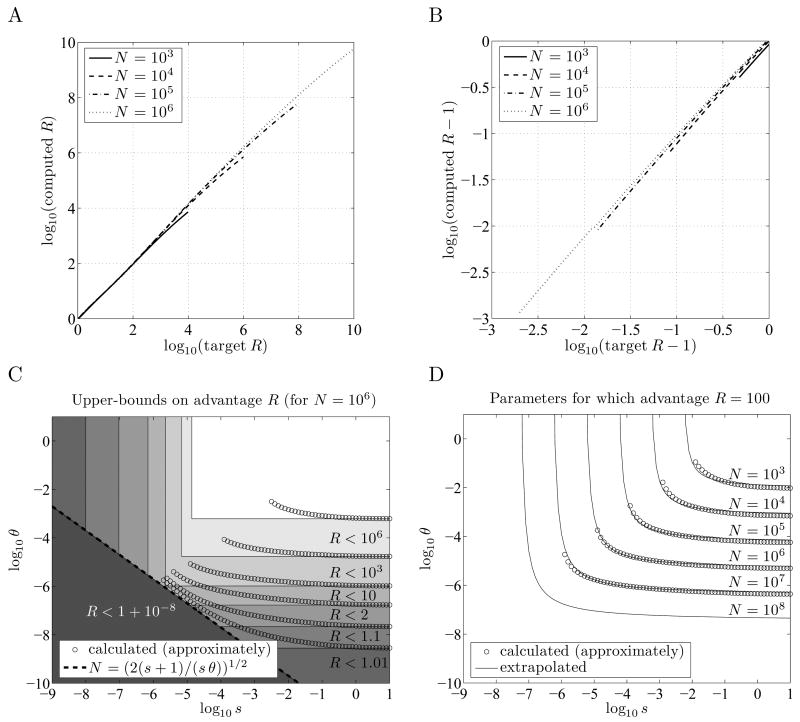
Figure 2.

Minimum conditions for bet-hedging to evolve in a finite population. R = p̂_fix (0, m̂_opt, N, θ, s) / p̂_fix (m̂,0, N, θ, s) denotes the estimated advantage provided by using the optimal bet-hedging strategy over using no bet-hedging. A and B: When $\theta =3\sqrt{(R-1)logR}/(N\text{log}N)$ (from Equation 6), s = ∞, and m−1−e^−θ ≈ m̂_opt, the ratio p̂_fix (0, m̂_opt, N, θ, s) / p̂_fix(m̂_opt, 0, N, θ, s) , shown on the vertical axis, is approximately R. Curves in A are shown for R < N²/100, and in B for R > 1 + 10 log(N)²/N, roughly the range for which the approximation is accurate. (Note that B covers the range from R = 1.001 to R = 2.) C: Rectangular regions in which s and θ must fall to allow for a given advantage R; these are necessary but not sufficient conditions. For smaller R these rectangles are encroached on by the approximate equation for N_min Computed estimates are shown for θ ≤ s. D: Estimated parameters θ and s for which R = 100, given as hyperbolas in log (s) and log(θ). Our computed estimates become less accurate for small sN and large θ, and are shown only for sN > 10. The curve for N = 10⁸ is extrapolated using Equation 7.