Figure - PMC

Skip to main content

An official website of the United States government

Here's how you know

Here's how you know

Official websites use .gov
A .gov website belongs to an official government organization in the United States.

Secure .gov websites use HTTPS
A lock ( ) or https:// means you've safely connected to the .gov website. Share sensitive information only on official, secure websites.

View full-text article in PMC

. 2006 Jun;127(6):719–735. doi: 10.1085/jgp.200509438

Search in PMC
Search in PubMed
View in NLM Catalog
Add to search

Copyright © 2006, The Rockefeller University Press

This article is distributed under the terms of an Attribution–Noncommercial–Share Alike–No Mirror Sites license for the first six months after the publication date (see http://www.rupress.org/terms). After six months it is available under a Creative Commons License (Attribution–Noncommercial–Share Alike 4.0 Unported license, as described at http://creativecommons.org/licenses/by-nc-sa/4.0/).

PMC Copyright notice

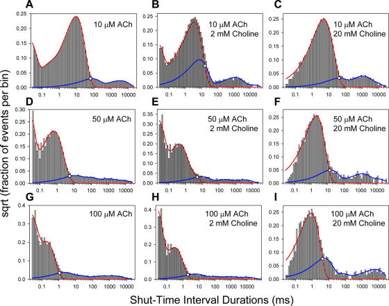
Figure 4. — Examples of experimentally obtained shut-time distributions, and calculation of t _crit values. For each histogram, the red and blue lines are the mixtures of exponential densities corresponding to the components to either side of the cut (see Materials and Methods). It can be shown that the t _crit for any given distribution (open circles) coincides with the time value at which these two exponential densities intersect (Eq. 3). The sum of the red and blue lines gives, of course, the mixture of exponential densities corresponding to all the components of the distribution (bear in mind, though, that the ordinates are plotted as the square root). The t _crit value, the total number of shuttings, and the fraction of misclassified shuttings in these example histograms are, respectively, as follows: A: 65.44 ms, 12,051, 0.008; B: 15.92 ms, 19,664, 0.124; C: 45.03 ms, 19,239, 0.012; D: 5.40 ms, 45,564, 0.007; E: 5.14 ms, 34,274, 0.008; F: 12.41 ms, 4,029, 0.022; G: 1.09 ms, 40,149, 0.009, H: 1.99 ms, 29,204, 0.004, I: 4.28 ms, 4,707, 0.054.