Figure 4.

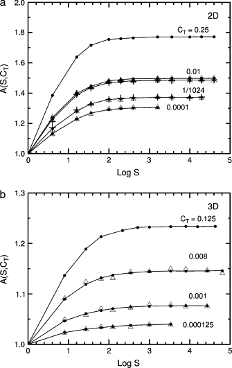
Dependence of the capture time on the number S of targets or sets of targets and traps for fixed target concentrations C_T. Values of A(S, C_T) are defined in Eq. 10. (a) Triangular and square lattices. (b) Cubic lattice. Note the changes in scale and C_T. Circles and lines, targets but no traps; triangles, traps and targets. The standard hierarchy of traps is used, 16/8/4/2/T, P_ESC = 0.1. In panel a for C_T = 0.01, the upper line is for the square lattice and the lower line is for the triangular lattice. Panel a also shows results for two alternative trap distributions on the triangular lattice, + for C_T = 0.01, the continuous distribution of Eq. 11, and + for C_T = 1/1024, the uniform discrete distribution 7/7/7/7/T. Runs were set up so that all concentrations and values of S were exact, although this limited the concentrations used. For example, when C_T = 0.01, the first series of runs had only target sites at a fixed concentration and the system size was varied. There was one target in a 10 × 10 grid, four targets in a 20 × 20 grid, and so forth to 3600 targets in a 600 × 600 grid. The second series used the same target concentrations and grids but one set of 30 traps per target, so the total concentration was C_Tt = 0.31. For runs with targets and traps, 500 trap configurations were used, and 1000 tracers per trap configuration. For runs with traps alone, to get smooth curves 1000 trap configurations were used and 10,000 tracers per trap configuration.