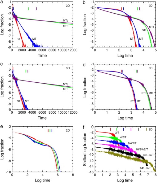
Figure 5.

Distribution of capture times from Monte Carlo calculations for the standard example, 16/8/4/2/T but with P_ESC = 0.2 so that all the curves can be shown conveniently on the same scale. Changes in noise levels within a curve are due to changes in bin width. Vertical lines at top, means. Notation in panels (a–d): ST (red), single target but no traps; MT (blue), multiple targets but no traps; STt (green), single set of traps and target; MTt (purple), multiple sets of traps and targets. (a) Log fraction versus time for two dimensions, grid size 10 × 10 for the ST and STt curves, and 320 × 320 for the MT and MTt curves. (b) The same data versus log time to show the power-law region in the STt and MTt curves. (c) Log fraction versus time for three dimensions, grid size 5 × 5 × 5 for the ST and STt curves, and 50 × 50 × 50 for the MT and MTt curves. (d) The same data versus log time. The MT and MTt curves are for 1024 sets in two dimensions and 1000 in three dimensions. (e) The standard hierarchy 16/8/4/2/T (red) gives a power-law region but the uniform discrete distribution 7/7/7/7/T (green) and the continuous uniform distribution (blue) give more complicated curves. All three runs were on a 30 × 30 triangular lattice, and 5 million repetitions were used instead of the usual 0.5 million to separate the histograms more cleanly. (f) Increasing the number of levels in the hierarchy increases the size of the power-law region. The hierarchies used are 2/T, 4/2/T, 8/4/2/T, 16/8/4/2/T, 32/…/2/T, and 64/…/2/T with P_ESC = 0.1. For clarity the curves are shifted downward by 0, 1, 2, 3, 4, and 5 units, respectively. One target and set of traps was used on a triangular lattice. The system size was varied between 8 × 8 and 66 × 66 to keep the trap concentration as constant as possible, 0.02972 ± 0.00098; that is, an SD of 3.28% of the mean.