
Figure 12.
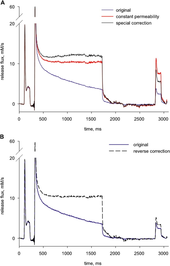
The “constant permeability” correction. (A) Blue trace:  ≲t
≲t
 , same as in Fig. 7 B. Red:
  c
c
 t
t
 , calculated according to Eq. 16. The choice of the value 14.5 mM for CaSR(0) led to a nearly constant corrected level during late portions of the conditioning pulse. Black: correction according to Eq. 17, with CaSR(0) = 11.5 mM and pump flux computed from the removal model, with best fit parameters given in the legend of Fig. 6. (B) Blue trace:
  ≲t
≲t
 , repeated from A. “Reverse correction” (black dashed) is obtained with Eq. 17, by increasing the term “pump flux” during the interval between conditioning and test, which increases the denominator in Eq. 17, until the corrected test release flux reaches the same steady level as the reference release flux (in accordance with the constant permeability hypothesis). An implausibly large 67% of the amount released during the conditioning pulse must return in order to reach this level.