Figure 7. The a-wave and the derived rod response at a range of early measurement times.

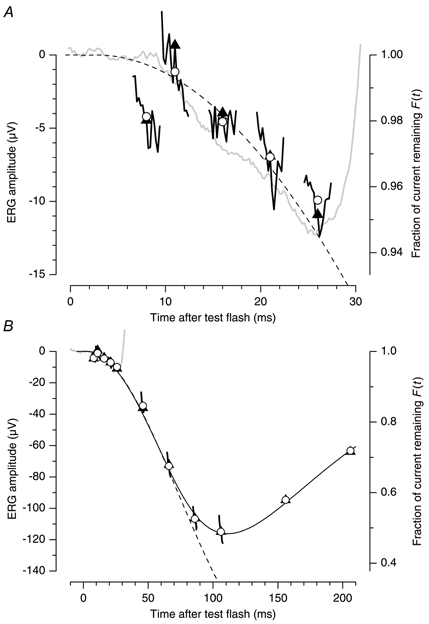
The ERG elicited by the test flash (grey trace) is compared with the rod response derived from the paired-flash results in Fig. 6. Each test-probe separation time, t_sep, in Fig. 6 leads to a ‘continuum’ trace for the derived rod response in this figure, where all measurements are plotted at the time after the test flash at which the probe response was measured, i.e. at t=t_sep+t_meas. These continuum traces are plotted over the window of measurement times t_meas from 4.6 to 7.4 ms, indicated by the inset in Fig. 6. ^, mean over this window; ▴, value at t_meas= 6 ms (i.e. at the centre of the window). The ordinate scale at the right plots the fractional probe response, exactly as in Fig. 6, i.e. F(t)=R_sep(t)/R_alone(t). The absolute scale at the left has been obtained as a_max(1 − F), where the maximal amplitude was obtained by fitting the family of a-wave responses, as a_max= −225 μV. The dashed trace plots the delayed Gaussian prediction of the model for pure activation, eqn (7a), with A= 5.4 s⁻², τ= 1 ms and t_d= 1.7 ms. The continuous trace plots eqn (6) using the same activation parameters, and t₀= 74 ms, τ_rec= 114 ms, and n = 8. A, expanded view at early times; B, full view, for measurements out to a test-flash separation of 200 ms. Additional details are given in legend to Fig. 6.