
Fig. 4.
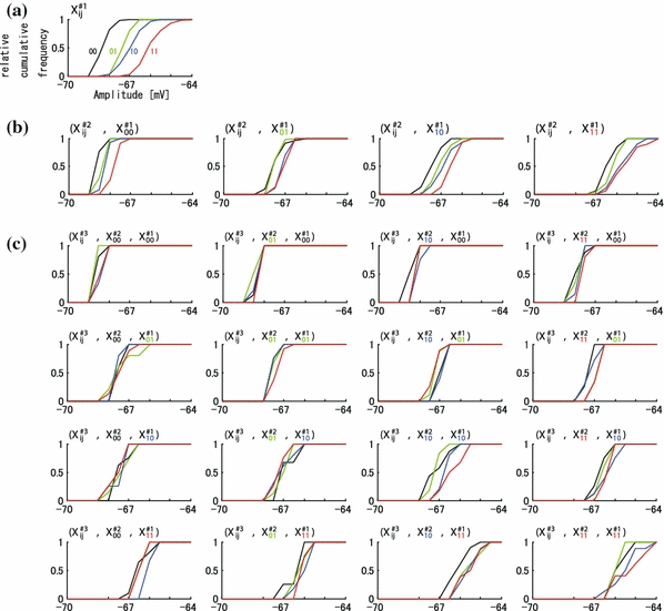
An example of distribution of membrane potentials by one, two, and three time history-steps in sub-threshold group. (a) Standardized cumulative histogram (SCH) of amplitude by the pattern of spatial input at one time-history step. The X-axis indicates the amplitudes (mV, referred also dotted lines in Fig. 2a). The colors of traces indicate the distribution of input spatial patterns: red, blue, green, and black traces indicate the spatial input pattern of “X#100”,“X#101”,“X#110”, and “X#111”, respectively. The Y-axis indicates standard cumulative frequency of amplitudes. (b) SCH by the pattern of spatial input at two time-history steps. The trace in (a) “X#100”,“X#101”,“X#110”, and “X#111” was further subclassified into “(X#2ij,X#100)” (left graph),“(X#2ij,X#101)” (middle left graph),“(X#2ij,X#110)” (middle right graph), and “(X#2ij,X#111)” (right graph) by the pattern at two time-history steps, respectively. In each graph, the distribution of the amplitudes by one time-history step is indicated by the color of the traces: black, green, blue, and red traces indicate the distribution of the response by “X#200”,“X#201”,“X#210”, and “X#211”, respectively. (c) SCH by the pattern of spatial input at three time-history steps. The graph in (b) “(X#2ij,X#100)”, “(X#2ij,X#101)”, “(X#2ij,X#110)”, and “(X#2ij,X#111)” was further subclassified into “(X#3ij,X#2ij,X#100)” (upper four graphs), “(X#3ij,X#2ij,X#101)” (upper middle four graphs), “(X#3ij,X#2ij,X#110)” (lower middle four graphs), and “(X#3ij,X#2ij,X#111)” (lower four graphs) in (c) by the pattern at three time-history steps, respectively. In each graph, the distribution of the amplitudes by three time-history steps is indicated by the color of the traces: black, green, blue, and red traces indicate the distribution of the response by “X#300”,“X#301”,“X#310”, and “X#311”, respectively