Figure 4. Relation of standard deviation and coefficient of variation with firing frequency.

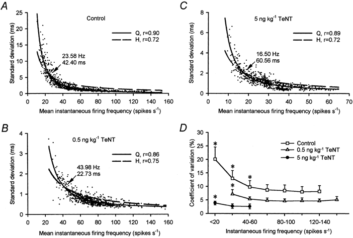
A, plots of the standard deviation versus the mean firing frequency of 857 stationary epochs obtained from 30 control motoneurones. The dashed line is the hyperbolic (H) function y = 143.8(0.2 + x)⁻¹ (r = 0.72; P < 0.001). The continuous line is the polynomial quadratic (Q) inverse function y = −0.2 + 51.5x + 2423.6x² (r = 0.90; P < 0.001). B, same as A, but for 770 fixations from 29 low-dose-treated motoneurones. The hyperbolic regression was y = 52.2(0.5 + x)⁻¹ (r = 0.75; P < 0.001). The polynomial regression was y = 0.2 + 1.3x + 1760.6x² (r = 0.86; P < 0.001).C, same as A, but for 775 fixations analysed in 28 high-dose-treated motoneurones. The hyperbolic function was y = 33.8(0.2 + x)⁻¹ (r = 0.72; P < 0.001). The polynomial regression was y = 0.2 + 8.2x + 426.1x² (r = 0.89; P < 0.001). In A-C, the point of crossing of both curves is shown (arrow) both in rate and interval units. D, mean coefficient of variation (in %) grouped for firing frequency intervals of 20 spikes s⁻¹ for 30 control (□), 29 low-dose- (▵) and 28 high-dose-treated (•) abducens motoneurones (error bars are s.d.). Asterisks indicate those firing intervals whose mean coefficient of variation was significantly different to the rest of firing intervals within the same treatment (two-way ANOVA, Scheffé's post hoc comparisons, P < 0.001).