
Figure 4. Virion heterogeneities can soften thresholds.
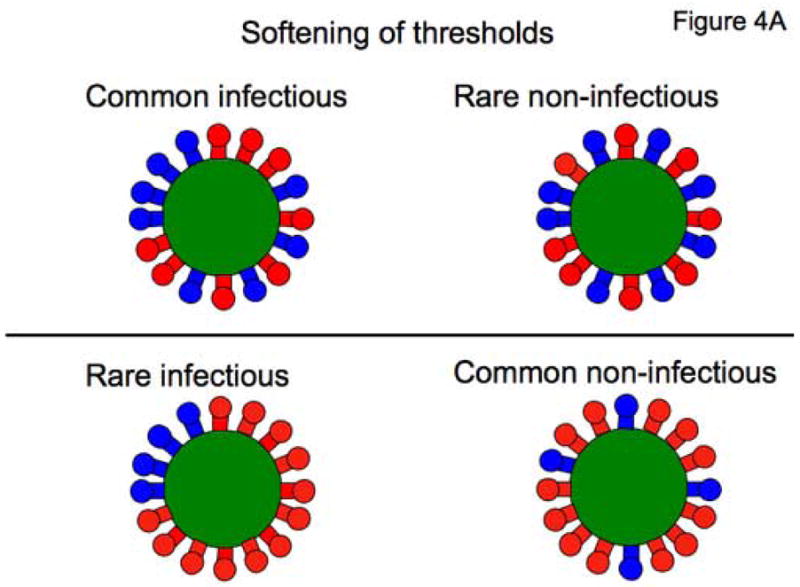
A. The cartoon shows how heterogeneity in Env distribution over virion spheres can soften threshold effects. The virions all have 16 trimers (active in blue, inert in red). In the top row, the virions have eight active trimers, in the bottom row, only four. If the condition for infectivity is a minimum of four contiguous trimers, infectivity will be common among the virions in the top row, but rare among those in the bottom row. Thus the number of active trimers will affect the probability that the requisite number will be present in a contiguous constellation conducive to infectivity; this scheme differs from the all-or-nothing effect of thresholds on infectivity that is determined solely by the number of active trimers regardless of how they are spread over the virion sphere. The consideration of spherical distribution causes a softening of the infectivity thresholds. Different spatial constellations of a the same number of contiguous trimers may also have different propensities to function in entry, a further blurring effect. In addition, any spare trimers that are outside entry-competent constellations could still modulate infectivity by contributing tp virus-cell attachment, creating yet more blurring of any simple threshold effect.
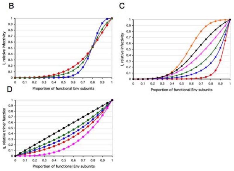
B. If the infectivity of the average virion is neither all-or-nothing nor exactly proportional to the number of functional trimers present, then a certain proportion of inert trimers would reduce the relative infectivity disproportionately without eliminating it. The infectivity may drop more precipitously in an intermediate zone than when the first and last trimers are knocked out. Such mixed liminal-incremental models assign different weights to each absolute-liminal equation. We assume n=9. Three curves for a soft threshold around L=5, I=(IL=1+bIL=2+b2IL=3+b4IL=4+b8IL=5+b4IL=6+b2IL=7+bIL=8+IL=9)/(2+2b+2b2+2b4+b8) are shown with a low (b=2) (blue squares), intermediate (b=1.3) (green triangles), and high (b=1.1) (red circles) degree of softness of the threshold.
C. Three curves with the same three values of b as in (B) for a low threshold around L=2, I=(b6IL=1+ b9IL=2+ b6IL=3+ b5IL=4+ b4IL=5+ b3IL=6+ b2IL=7+ bIL=8+ IL=9)/(1+b+b2+b3+b4+b5+2b6+b9) (b=2, red circles; b=1.3, blue squares; b=1.1, green triangles) and three for a high threshold around L=8, I=(IL=1+bIL=2+b2IL=3+b3IL=4+b4IL=5+b5IL=6+b6IL=7+b9IL=8+b6IL=9)/(1+b+b2+b3+b4+b5+2b6+b9) (b=2, orange circles; b=1.3, black squares; b=1.1, magenta triangles).
D. The blending of the two most realistic models at the trimer level, S=1 and the protomer-incremental one, is shown. Five different curves on the spectrum between the two extremes are shown for values of the parameter h=0 (magenta circles), h=0.33 (red circles), h=0.5 (blue circles) h=0.67 (green circles) and h=1 (black circles). Note that unlike in the other diagrams, the y axis here represents the relative trimer function, q.