Figure 5. Empirical fit of combined liminal-incremental modeling at both trimer and virion levels.

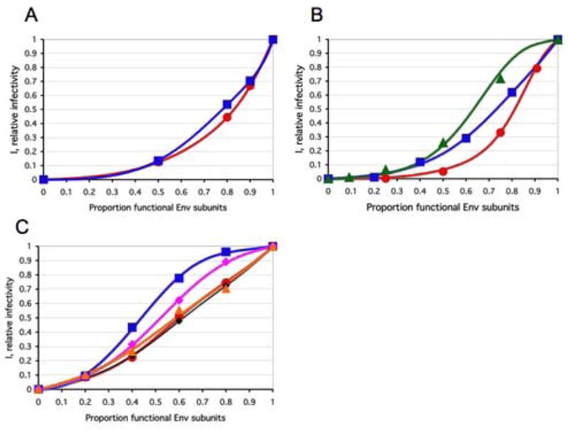
The optimized liminal-incremental models presented in Table 3 are illustrated graphically. Here n=9 throughout. A. The infectivity, I, of virus with mixed antigenic and non-antigenic Env in the presence of an excess of NAb (Yang et al., 2005a) is expressed on the y-axis as a function of the proportion of functional Env on the x-axis. The red curve for the function with a soft threshold around L=2 is shown to fit the data for the TCLA virus HXBc2 (mean of I for 8 NAbs, red circles). The blue curve for the function with threshold peaks at L=[1,7,8] is shown to fit the data for the PIs YU2, ADA and KB9 (mean of pooled I for 2–3 NAbs, blue squares). B. The infectivity, I, of virus with mixed cleavage-defective and functional Env is plotted on the y-axis with the proportion of cleavable Env on the x-axis. The red curve shows how well a function with a gradual threshold around L=[4,5] fits the data for the TCLA virus HXBc2 (Herrera et al., 2006) (red circles); the blue curve represents the function with a gradual threshold around L=7 to fit the data for the PI YU2 (Yang et al., 2005b) (blue squares); the green curve shows how the function with a threshold of around L=6 fits the data for the PI JR-FL (Herrera et al., 2006) (green triangles).

C. The infectivity, I, is plotted on the y-axis as a function of the proportion of active Env on the x-axis for virus with mixed mutant and wild-type Env, where the mutant is defective in CD4 binding, co-receptor interaction or in the fusion function of gp41 (Yang et al., 2006a). The liminal-incremental model curves are shown to fit the data points of the same color: The TCLA virus HXBc2 defective in binding CD4, L around 8 (red, circles) or CXCR4, L around 8 (black, diamonds); PIs defective in binding CD4, L around 7 (blue, squares) or CCR5, L around 5 (magenta, diamonds); PIs defective for gp41 fusion function, L around 8 (orange, triangles). As shown in Supplementary Table 2, L around 5 can fit all these five data sets well with concomitantly high h values. L around 8 can also fit all five well and then the h values are lower. This compensatory effect of the two soft threshold levels is also seen among the individual five models in Table 3.