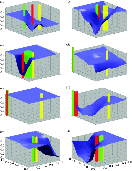
Figure 3.

Victim-cue (e.g. host plants) phenotypes and exploiter-response phenotypes (e.g. phytophagous insects) are plotted above the two-dimensional signal space. The two bottom axes represent signal strengths of cue phenotype. The surface shows the average response of all exploiters to a hypothetical signal at any point in the signal space. The vertical columns represent victim clusters: medium grey, undefended; light grey, intermediate; and dark grey, defended. The centre of each column is at the average of the victim cue-phenotypes in the cluster in question and the radius is the standard deviation. The images are captured after a simulation of exploiter–victim coevolution. (a) The simulation is initialized with the plants lined up on the diagonal. The insects have learnt to respond to the plants; two specialists, one on each edible plant, have evolved (not seen in figure). (b) The most edible plant cluster has approached the noxious plant cluster. The runaway movement with the most edible plant following the least edible one has started. (c) The chase moves to the border of the signal space. The intermediate plant is following behind. (d) The chase has been arrested in a corner, and the intermediate plant has been left behind. (e) The insects have stopped discriminating between plants. (f) The two plants in the corner have drifted apart owing to the lack of selection on signals. Becoming separated, the insects are now starting to discriminate between plants again. The chase has been re-initiated. (g) The chase has been moving towards the centre and attracted all plants in the middle. (h) The chase is now continued towards a border of the signal space and the procedure repeats from (c) and onwards (Norrström et al. 2006).