Figure 6. Tests of the quality of the fit produced in a single simulated experiment of the same sort as the 1000 simulations used to generate Figs 3–5.

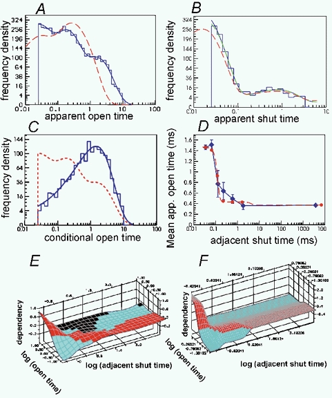
A, histogram of distribution of apparent (‘observed’) open times with a resolution of 25 μs. The solid blue line shows the HJC open time distribution predicted by the fitted values of the rate constants with a resolution of 25 μs. Dashed red line: the open time distribution predicted by the fitted values of the rate constants without allowance for limited resolution - the estimate of the true open time distribution. B, as in A but for apparent shut times (note that only shut times up to t_crit= 3.5 ms are used for fitting so only these appear in the histogram). The HJC distribution is, as always, calculated from the exact expressions up to 3t_res (i.e. up to 75 μs in this case), and thereafter from the asymptotic form. Green line: the asymptotic form plotted right down to t_res= 25 μs. It is seen to become completely indistinguishable from the exact form for intervals above about 40 μs. C, histogram of distribution of ‘observed’ open times with a resolution of 25 μs for openings that are adjacent to short shuttings (durations between 25 and 100 μs). Solid line: the corresponding HJC conditional open time distribution predicted by the fitted values of the rate constants with a resolution of 25 μs. Dashed line: the HJC distribution of all open times (same as the solid line in A). D, conditional mean open time plot. The solid diamonds show the observed mean open time for apparent openings (resolution 25 μs) that are adjacent to apparent shut times in each of seven shut time ranges (plotted against the mean of these shut times). The bars show the standard deviations for each mean. The shut time ranges used were (ms) 0.025–0.05, 0.05–0.1, 0.1–0.2, 0.2–2, 2–20, 20–200 and > 200. Note, however, that shut time greater than t_crit (3.5 ms) will be shorter than predicted if there was more than one channel in the patch so the values on the abscissa above 3.5 ms are unreliable. The solid circles show the corresponding HJC conditional mean open times predicted by the fitted values of the rate constants with a resolution of 25 μs, for each of the seven ranges. The dashed line shows the continuous HJC relationship between apparent mean open times conditional on being adjacent to the shut time specified on the abscissa. E, ‘observed’ dependency plot for apparent open times and adjacent shut times (resolution 25 μs). Regions of positive correlation (dependency greater than zero) are red, negative correlations are blue, and black areas indicate regions where there were not enough observations to plot. F, fitted HJC dependency plot, predicted by the fitted values of the rate constants with a resolution of 25 μs.