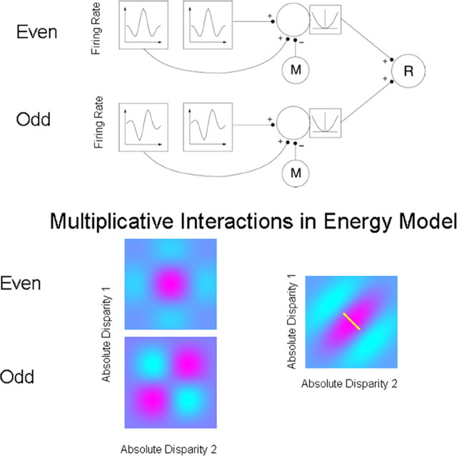
Figure 2.

Adaptation of the disparity energy model to compute relative disparity. Top, Inputs whose firing rates are selective for absolute disparity, similar to those found in V1, are summed and squared. Relative disparity is computed by applying a second-level disparity energy computation to the outputs of the two V1-like receptive field. Each first-level disparity energy model computes absolute disparity. Such responses are summed, squared, and pooled to produce a consistent selectivity for relative disparity (neuron R). One aspect of this implementation is that the output from monocular filters (M) is subtracted from the neuronal signal before the squaring operation. If this monocular term is not subtracted, the response is more strongly influenced by absolute disparity. (Reproduced with permission from Thomas et al., 2002, their Fig. 5.) Bottom, The spatial structure underlying the model. This shows the combinations arising from two pairs of neurons sensitive to absolute disparity. A pair of neurons tuned with even symmetry for absolute disparity are summed together with a pair of neurons tuned with odd symmetry for absolute disparity. On each plot, relative disparity is a constant difference between two absolute disparities, indicated by the small white line on the far right plot. The interactions provided by the energy model provide for a consistent selectivity to relative disparity over a range of different absolute disparities. This local invariance of response is an important new property that provides for a context-dependent response to combinations of absolute and relative disparity.