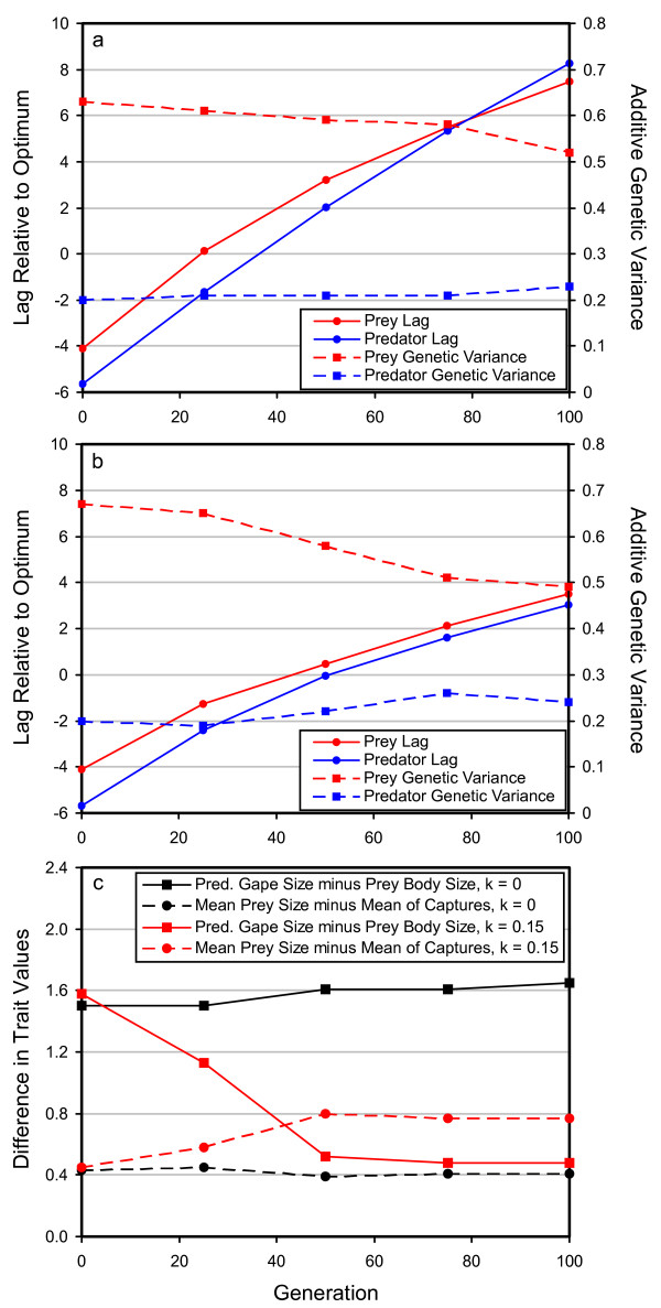
Figure 4.

Mechanistic details of the predator-prey model for a sample set of parameter values. The top two panels show the lag and additive genetic variance over time in the predator-prey model for the two species in typical control (a) and experimental (b) runs of the simulation. When the predator-prey interaction is absent, the lag for both species increases rapidly (a). However, when the predator-prey interaction is present, the rate of increase of the lag is reduced for both species, permitting both species to persist for longer periods of time before extinction (b). Under these parameter combinations, the reduced lag occurs for both the predator (solid blue lines) and the prey (solid red lines). The additive genetic variances of the predator (broken blue lines) and prey (broken red lines) do not differ dramatically between the experimental and control runs, except that there is a slightly more rapid loss of genetic variance in the prey during the experimental runs. The bottom panel (c) shows the tendency for the predator to eat the most maladapted individuals as the optimum moves. When the optimum does not move (black lines), the difference between mean predator gape size and mean prey body size reaches a steady-state expected value. A similar situation occurs for the difference between the mean size of prey in the population and the mean size of prey that are actually eaten. As the optimum moves (red lines), however, the gape size of the predator decreases relative to the mean prey size, and the difference in size between mean prey size and predated individuals becomes even greater than it is in the population experiencing a stationary optimum. The results depicted in this figure used the standard set of parameter values (see methods), and k and ω² were set to 0.15 and 50, respectively. Each point on each graph is a mean from 50 replicate runs of the simulation.