Constrained Least Absolute Deviation Neural Networks

Abstract

It is well known that least absolute deviation (LAD) criterion or L₁-norm used for estimation of parameters is characterized by robustness, i.e., the estimated parameters are totally resistant (insensitive) to large changes in the sampled data. This is an extremely useful feature, especially, when the sampled data are known to be contaminated by occasionally occurring outliers or by spiky noise. In our previous works, we have proposed the least absolute deviation neural network (LADNN) to solve unconstrained LAD problems. The theoretical proofs and numerical simulations have shown that the LADNN is Lyapunov-stable and it can globally converge to the exact solution to a given unconstrained LAD problem. We have also demonstrated its excellent application value in time-delay estimation. More generally, a practical LAD application problem may contain some linear constraints, such as a set of equalities and/or inequalities, which is called constrained LAD problem, whereas the unconstrained LAD can be considered as a special form of the constrained LAD. In this paper, we present a new neural network called constrained least absolute deviation neural network (CLADNN) to solve general constrained LAD problems. Theoretical proofs and numerical simulations demonstrate that the proposed CLADNN is Lyapunov stable and globally converges to the exact solution to a given constrained LAD problem, independent of initial values. The numerical simulations have also illustrated that the proposed CLADNN can be used to robustly estimate parameters for nonlinear curve fitting, which is extensively used in signal and image processing.

I. Introduction

The use of the least absolute deviation (LAD) or L₁-norm criterion provides in many applications in signal and image processing a useful and reliable alternative to the least squares (LS) criterion (L₂-norm) or Chebyshev criterion (L_∞-norm). These applications span the field of deconvolution, state estimation, blind source separation, system identification, parameter estimation, time-frequency analysis, and time-delay estimation [1]-[13]. The L₁-norm solutions of systems of linear algebraic equations have certain properties not shared by the ordinary LS (L₂-norm) solutions [1]-[13] as follows. 1) An L₁-norm solution of an overdetermined system of linear equations always exists although the L₁-norm solution is not necessarily unique in contrast to the L₂-norm solution where the solution is always unique when matrix A is of full rank. 2) L₁-norm solutions are robust which means the solution is resistant (insensitive) to some large changes in the data. This is an extremely useful property when the data are known to be contaminated by occasional wild points or spiky noise. 3) For fitting a number of data points by a constant, the L₁-norm estimate can be interpreted as the median while the L₂-norm estimate is the mean. A general LAD with equality and inequality constraints are formulated as follows:

$$\{\begin{array}{ll}\mathrm{Minimize}& {\Vert \mathit{Ax}-b\Vert }_1\\ \mathrm{Subject\; to}& C^{T}x=d,E^{T}x\le f\end{array}$$ (1)

where A = [a_ij] ∈ R^{M × N}, b ∈ R^M, C = [c_ij] ∈ R^{N × P}, d ∈ R^P, E = [c_ij] ∈ R^{N × Q}, f ∈ R^Q, and x ∈ R^N is the solution to be determined.

Because of its excellent properties, the LAD optimization model described by (1) has been extensively studied [1]-[10] and many numerical algorithms for solving this model, such as Simplex and Karmarkar’s algorithms, have been proposed [7]-[9]. However, with the increase of the model scale, these numerical algorithms are not adequate for solving real-time problems. One possible and promising approach to real-time optimization is to apply neural networks (NNs). Because of the inherent massive parallelism, the NN-based approach can solve optimization problems within a time constant of the network, for example, several milliseconds. Hopfield and Tank first proposed to use an NN for solving linear programming problems [14], [15]. Their creative work has motivated many researchers to investigate alternative NNs for solving linear and nonlinear programming problems [1], [2], [11]-[13], [16]-[22] and for solving arbitrary roots of polynomials [23], [24]. For instance, Cichocki and Unbehauen proposed to use an NN for solving the unconstrained LAD problem [1]. In the NN proposed by Cickocki and Unbehauen for implementing the LAD optimization model, some complex control circuits, such as “inhibition control circuits” and “switch control circuits,” were introduced [1]. This made their NN models complicated and difficult for implementation. For some so-called ill-conditioned problems, their network parameters have to be adjusted, which is unrealistic for practical applications since the exact solutions are unknown. In our previous work, we presented a new NN to solve the unconstrained LAD optimization model [11], [12]. This NN can be implemented by using a number of adders, limiters, and integrators, without any control circuits to be tuned. By mathematical proofs and experimental validations, the proposed unconstrained LAD network is Lyapunov stable and able to converge globally to the exact solution to a given problem. In this paper, we propose another NN to solve the constrained LAD optimization problem, which can be viewed as the generalization of the unconstrained LAD because when the constraints are set to zeros, the constrained LAD model described by (1) is equivalent to an unconstrained LAD model. Likewise, the NN for solving constrained LAD problems, namely, CLADNN, can be implemented without any control circuits and its convergence is proven theoretically and validated experimentally.

The rest of this paper is organized as follows. In Section II, preliminary theories are given, which will be cited in later sessions. In Section III, the LAD NN with equality constraints is presented first and then it is extended to the general case where the equality and inequality constraints exist simultaneously. Section IV presents three groups of numerical experiments for the validation of the convergence performances of the proposed CLADNN. Finally, the conclusions are given in Section V.

II. Preliminary Theories and Definitions

In this section, the necessary mathematical definitions and lemmas are introduced, which will be used to describe the proposed LAD NN in Section II-A.

Definition 1 (Lipschitz Continuous [21], [25])

The mapping F : Ω ⊂ R^N is said to be Lipschitz continuous with a positive constant L on the set Ω, if for each pair of points x, y ∈ Ω, the following inequality holds:

$${\left|F(\mathbf{x})\mathbf{-}F\left(\mathbf{y}\right)\right|}_2\le L{\left|\mathbf{x}\mathbf{-}\mathbf{y}\right|}_2$$

Definition 2 (Lyapunov Stable [21], [26]-[29])

Let x(t) be a solution of the dynamic system x˙ = f(x) ((dx/dt) = f(x). The equilibrium point x*, that is f(x*) = 0, is defined to be Lyapunov stable if, for any x₀ = x(t₀) and scalar ε > 0, there exists δ > 0 such that if ‖x(t₀) − x*‖₂ < δ, then ‖x(t) − x*‖₂ < ε for all t > t₀.

Definition 3 (Global Convergence [21], [26]-[29])

An NN is said to be globally convergent if for any initial point taken in the definition domain, every trajectory of the corresponding dynamic system converges to its unique equilibrium point.

Lemma 1 (Extended Brouwer’s Fixed Theorem [30, Th. 2.5])

Let Ω ⊂ R^N be compact and convex and let F : Ω → Ω be continuous. Then, F admits a fixed point.

Lemma 2

If f(x) and g(x) are Lipschitz continuous on Ω ⊂ R^N, then, for any constant k₁ and k₂, k₁ f(x) + k₂g(x) is also Lipschitz continuous on Ω ⊂ R^N.

Proof

See [11].

Lemma 3 (LaSalle’s Theorem [28, Th. VI])

Let V(x) be a scalar function with continuous first partial derivations. Let Ω_l designate the region where V(x) < l. Assume that Ω_l is bounded and that within Ω_l

$$V(\mathbf{x})<0\mathrm{for}\mathbf{x}\ne 0$$ (2.a)

$$\dot{V}(\mathbf{x})=\frac{\mathit{dV}(\mathbf{x})}{\mathit{dt}}\le 0.$$ (2.b)

Let R be the set of all points within Ω_l where V̇ (x) = 0 and let M be the largest invariant subset in R. Then, every solution x(t) in Ω_l tends to M as t → +∞.

III. Theories of CLADNNs

A. Theories of an NN of the LAD With Equality Constraints

We first construct an NN to solve the LAD problem only with equality constraints and prove its global convergence. This LAD problem is formulated as

$$\{\begin{array}{ll}\mathrm{Minimize}& {\Vert \mathbf{Ax}\mathbf{-}\mathbf{b}\Vert }_1\\ \mathrm{Subject\; to}& {\mathbf{C}}^T\mathbf{x}=\mathbf{d}\end{array}.$$ (3)

Using Proposition 1, we turn the problem described in (3) into another form, which is easier to solve.

Proposition 1

The optimization model described in (3) is equivalent to the following optimization model:

$$\{\begin{array}{ll}\mathrm{Minimize}& \{{\max }_{y\in \Omega }\{{\mathbf{y}}^T(\mathbf{Ax}\mathbf{-}\mathbf{b})\}\}\\ \mathrm{Subject\; to}& {\mathbf{C}}^T\mathbf{x}=\mathbf{d}\end{array}$$ (4)

where Ω = {ω ∈ R^M ‖ω_i| ≤ 1, i = 1, 2, …, M} ⊂ R^M.

Proof

For (4), we only need to prove ${\left|\mathbf{Ax}\mathbf{-}\mathbf{b}\right|}_1=\underset{\mathbf{y}\in \mathrm{\Omega }}{\max }\{{\mathbf{y}}^T(\mathbf{Ax}\mathbf{-}\mathbf{b})\}$. Let u = (Ax − b) ∈ R^M; then, for any y ∈ Ω, and i = 1, 2, …, M, we have |y_i| ≤ 1, thus

$${\mathbf{y}}^T(\mathbf{Ax}\mathbf{-}\mathbf{b})={\mathbf{y}}^T\mathbf{u}=\sum _{i=1}^M{y}_i{u}_i\le \sum _{i=1}^M|y_i|·|u_i|\le \sum _{i=1}^M|u_i|={\Vert \mathbf{Ax}\mathbf{-}\mathbf{b}\Vert }_1.$$

Specifically, let y⁰ = [sign(u₁), …, sign(u_M)]^T; then, y⁰ ∈ Ω and

$${({\mathbf{y}}^0)}^T(\mathbf{Ax}\mathbf{-}\mathbf{b})=\sum _{i=1}^M\mathrm{sign}(u_i)u_i=\sum _{i=1}^M|u_i|={\Vert \mathbf{Ax}\mathbf{-}\mathbf{b}\Vert }_1.$$

Thus

$$\underset{\mathbf{y}\in \mathrm{\Omega }}{\mathrm{Max}}{\mathbf{y}}^T(\mathbf{Ax}\mathbf{-}\mathbf{b})={\Vert \mathbf{Ax}\mathbf{-}\mathbf{b}\Vert }_1.$$

This completes the proof of Proposition 1.

Now, we propose an NN for solving the problem in (4) whose model is described by the following dynamic system:

$$\{\begin{array}{l}\frac{d\mathbf{x}}{\mathit{dt}}=\mathbf{-}\mathbf{C}({\mathbf{C}}^T\mathbf{x}\mathbf{-}\mathbf{d}\mathbf{-}\mathbf{z})\mathbf{-}{\mathbf{A}}^T{\mathbf{P}}_{\mathrm{\Omega }}(\mathbf{y}+\mathbf{Ax}\mathbf{-}\mathbf{b})\\ \frac{d\mathbf{y}}{\mathit{dt}}=\mathbf{-}(\mathbf{A}{\mathbf{A}}^T+\mathbf{I})\mathbf{y}+{\mathbf{P}}_{\mathrm{\Omega }}(\mathbf{y}+\mathbf{Ax}\mathbf{-}\mathbf{b})+\mathbf{ACz}\\ \frac{d\mathbf{z}}{\mathit{dt}}=\mathbf{d}\mathbf{-}{\mathbf{C}}^T[\mathbf{x}\mathbf{-}{\mathbf{A}}^T\mathbf{y}+\mathbf{Cz}]\end{array}$$ (5)

where x ∈ R^N, y ∈ R^M, z ∈ R^P, Ω = {ω ∈ R^M‖ω_i| ≤ 1,i = 1, 2, …, M} ⊂ R^M, A = [a_ij] ∈ R^{M × N}, C = [ c_ij] ∈ R^{N × P}, b ∈ R^M, and d ∈ R^P. I is a unit matrix of R^{M × M}. For any given vector ξ = [ξ₁, ξ₂, …, ξ _M]^T ∈ R^M, P_Ω (ξ) = [P_Ω (ξ₁), P_Ω (ξ₂), …, P_Ω(ξ_M)]^T ∈ Ω, where P_Ω(·) is a projection operator and for i = 1, 2 …, M, P_Ω (ξ_i) is defined as

$$P_{\mathrm{\Omega }}({\xi }_i)=\frac{1}{2}(|{\xi }_i+1|\mathbf{-}|{\xi }_i\mathbf{-}1|)=\{\begin{array}{l}1,\\ {\xi }_i,\\ \mathbf{-}1,\end{array}\begin{array}{l}\mathrm{if}{\xi }_i>1\\ \mathrm{otherwise}.\\ \mathrm{if}{\xi }_i<\mathbf{-}1\end{array}$$ (6)

Since the NN described in (5) is a continuous-time network governed by a set of ordinary differential equations, it can be real-time implemented via very large scale integration (VLSI) complimentary metal–oxide–semiconductor (CMOS) circuits. In such a circuit implementation, the projection operator of P_Ω (·) is actually a simple limiter with a unit threshold. The matrix or vector multiplications are actually the synaptic weighting and summing operations, and hence, they can be implemented via a number of adders with a weighting function [1], [2], [11]-[13], [20]-[22], [31]-[33]. The rest are a number of simple integrators. The most important thing is that the architecture of the proposed network, as shown in Fig. 1, does not contain any control unit circuits or variable parameters to be tuned, which are usually found in the literature, e.g., in [1], [16], and [17], and thus its implementation becomes much easier. To conduct numerical validations, Fig. 2(a) illustrates the simulation circuit of the proposed network under MATLAB SIMULINK. In the following, we will prove that the NN described in (5) globally converges to the exact solution to problem (4), or equivalently, to problem (3).

Fig. 1.

Architecture of the CLADNN.

Fig. 2.

MATLAB SIMULINK simulator of the CLADNN. (a) Simulator architecture. (b) Solution convergence process for solving problem 1 (linear fitting).

Theorem 1

Suppose that the problem in (4) has a solution, then the NN described by (5) is Lyapunov stable and globally converges to the exact solution to problem (4).

Theorem 1 is proven as follows. First, we begin with the proofs of a number of propositions.

Proposition 2

Let Ω ⊂ R^N denote a closed convex set and let v = P_Ω (u) denote the projection of u on Ω, i.e., for each u ∈ R^N, there is a unique v ∈ Ω such that

$${\Vert \mathbf{u}\mathbf{-}\mathbf{v}\Vert }_2={\Vert \mathbf{u}\mathbf{-}{\mathbf{P}}_{\mathrm{\Omega }}(\mathbf{u})\Vert }_2=\underset{{\mathbf{u}}^{\ast }\in \mathrm{\Omega }}{\inf }{\Vert \mathbf{u}\mathbf{-}{\mathbf{u}}^{\ast }\Vert }_2$$

if and only if for all u* ∈ Ω, (u − P_Ω (u))^T (P_Ω(u) − u*)≥ 0.

Proof

See [11].

Proposition 3

Let Ω ⊂ R^N denote a closed convex set and let v = P_Ω (u) ∈ Ω denote the projection of u ∈ R^N on Ω. Then, the projection operator P_Ω (·) satisfies

$${\Vert {\mathbf{P}}_{\mathrm{\Omega }}(\mathbf{u})\mathbf{-}{\mathbf{P}}_{\mathrm{\Omega }}(\overline{\mathbf{u}})\Vert }_2\le {\Vert \mathbf{u}\mathbf{-}\overline{\mathbf{u}}\Vert }_2\mathrm{for}\mathbf{u},\overline{\mathbf{u}}\in {\mathbf{R}}^N.$$

That is, P_Ω (·) is Lipschitz continuous.

Proof

See [11].

Proposition 4

Let Ω ⊂ R^N be compact and convex, F : Ω ⊂ R^N → R^N be a continuous mapping, and P_Ω (ξ) be the projection of ξ ∈ R^N on Ω. Then, there exists a u* ∈ Ω so that (u − u*)^T F(u*) ≥ 0 for for all u ∈ Ω if and only if u*= P_Ω(u* − F(u*)).

Proof

See [11].

Proposition 5

If x* ∈ R^N is a solution to the problem in (4), then there exist y* ∈ Ω and z* ∈ R^P such that (x*, y*, z*) satisfies

$$\{\begin{array}{l}{\mathbf{C}}^T{\mathbf{x}}^{\ast }=\mathbf{d}\\ {\mathbf{y}}^{\ast }={\mathbf{P}}_{\mathrm{\Omega }}\left({\mathbf{y}}^{\ast }+{\mathbf{Ax}}^{\ast }\mathbf{-}\mathbf{b}\right)\\ {\mathbf{Cz}}^{\ast }={\mathbf{A}}^T{\mathbf{y}}^{\ast }\end{array}$$ (7)

where matrices A and C, vectors b and d, compact and convex set Ω, and projection operator P_Ω(·) have identical definitions as given in (6).

Proof

Let L(x, y, z) denote the Lagrange function of Max–Min optimization model in (4); then

$$L(\mathbf{x},\mathbf{y},\mathbf{z})={\mathbf{y}}^T(\mathbf{Ax}\mathbf{-}\mathbf{b})+{\mathbf{z}}^T(\mathbf{d}\mathbf{-}{\mathbf{C}}^T\mathbf{x}).$$ (8)

According to the Kuhn–Tucker (K–T) theorem [2], [26], we know that (x*, y*, z*) is a solution to convex optimization model (4) if and only if there exists a saddle point of model (4), (x*, y*, z*) ∈ R^N × Ω × R^P which satisfies

$$L({\mathbf{x}}^{\ast },\mathbf{y},{\mathbf{z}}^{\ast })\le L({\mathbf{x}}^{\ast },{\mathbf{y}}^{\ast },{\mathbf{z}}^{\ast })\le L(\mathbf{x},{\mathbf{y}}^{\ast },{\mathbf{z}}^{\ast })\forall \mathbf{x}\in {\mathbf{R}}^N\forall \mathbf{z}\in {\mathbf{R}}^P,\mathbf{y}\in \mathrm{\Omega }$$ (9a)

$$L({\mathbf{x}}^{\ast },{\mathbf{y}}^{\ast },\mathbf{z})\le L({\mathbf{x}}^{\ast },{\mathbf{y}}^{\ast },{\mathbf{z}}^{\ast })\le L(\mathbf{x},{\mathbf{y}}^{\ast },{\mathbf{z}}^{\ast })\forall \mathbf{x}\in {\mathbf{R}}^N\forall \mathbf{z}\in {\mathbf{R}}^P,\mathbf{y}\in \mathrm{\Omega .}$$ (9b)

$$L({\mathbf{x}}^{\ast },\mathbf{y},{\mathbf{z}}^{\ast })\le L({\mathbf{x}}^{\ast },{\mathbf{y}}^{\ast },{\mathbf{z}}^{\ast })\mathrm{yields}{\mathbf{y}}^T({\mathbf{Ax}}^{\ast }\mathbf{-}\mathbf{b})\le {{(\mathbf{y}}^{\ast })}^T({\mathbf{Ax}}^{\ast }\mathbf{-}\mathbf{b})$$ (10)

which is equivalent to

$${(\mathbf{y}\mathbf{-}{\mathbf{y}}^{\ast })}^T({\mathbf{b}\mathbf{-}\mathbf{Ax}}^{\ast })\ge 0\forall \mathbf{y}\in \mathrm{\Omega }.$$ (11)

In Proposition 4, let u = y, u* = y*, and F(u*) = b − Ax*; we immediately obtain

$${\mathbf{y}}^{\ast }={\mathbf{P}}_{\mathrm{\Omega }}({\mathbf{y}}^{\ast }+{\mathbf{Ax}}^{\ast }\mathbf{-}\mathbf{b}).$$ (12)

L(x*, y*, z) ≤ L(x*, y*, z*) yields

$${\mathbf{z}}^T({\mathbf{d}\mathbf{-}\mathbf{C}}^T{\mathbf{x}}^{\ast })\le {({\mathbf{z}}^{\ast })}^T({\mathbf{d}\mathbf{-}\mathbf{C}}^T{\mathbf{x}}^{\ast }).$$ (13)

Utilizing the fact that inequality (13) must hold for all z ∈ R^P, we obtain

$${\mathbf{C}}^T{\mathbf{x}}^{\ast }=\mathbf{d}.$$ (14)

L(x*, y*, z*) ≤ L(x, y*, z*) yields

$${{(\mathbf{A}}^T{\mathbf{y}}^{\ast }\mathbf{-}{\mathbf{Cz}}^{\ast })}^T{\mathbf{x}}^{\ast }\le {{(\mathbf{A}}^T{\mathbf{y}}^{\ast }\mathbf{-}{\mathbf{Cz}}^{\ast })}^T\mathbf{x}.$$ (15)

Utilizing the fact that inequality (15) must hold for all x ∈ R^N, we obtain

$${\mathbf{Cz}}^{\ast }={\mathbf{A}}^T{\mathbf{y}}^{\ast }.$$ (16)

Conversely, if (x*, y*, z*) ∈ R^N × Ω × R^P satisfies (7), then (9a) and (9b) hold for all x ∈ R^N, and y ∈ Ω and z ∈ R^P. This completes the proof of Proposition 5.

Corollary

For any y ∈ R^M and P_Ω(ξ) = 1/2 (|ξ + 1| − |ξ −1 |), the following inequality holds:

$${({\mathbf{P}}_{\mathrm{\Omega }}(\mathbf{y}+\mathbf{Ax}\mathbf{-}\mathbf{b})\mathbf{-}{\mathbf{y}}^{\ast })}^T(\mathbf{b}\mathbf{-}{\mathbf{Ax}}^{\ast })\ge 0.$$ (17)

Proof

Let u = (y + Ax − b) ∈ R^M , then P_Ω(u) ∈ Ω, i.e., |P_Ω(u_i)| ≤ 1 for i = 1, 2, …, M. Since (11) holds for all y ∈ Ω (|y_i| ≤ 1, i = 1, 2, …, M), thus (17) obviously holds. [Note: (17) holds for all y ∈ R^M, whereas (11) holds only for all y ∈ Ω.]

For convenience of proving Theorem 1, we rewrite dynamic system (5) into the following form:

$${\left(\frac{d\mathbf{x}}{\mathit{dt}}\frac{d\mathbf{y}}{\mathit{dt}}\frac{d\mathbf{z}}{\mathit{dt}}\right)}^T=\mathbf{-}\mathbf{F}(\mathbf{x}\mathbf{,}\mathbf{y}\mathbf{,}\mathbf{z})$$

where

$$\mathbf{F}(\mathbf{x},\mathbf{y},\mathbf{z})=\left(\begin{array}{c}{\mathbf{C}(\mathbf{C}}^T\mathbf{x}\mathbf{-}\mathbf{d}\mathbf{-}\mathbf{z})+{\mathbf{A}}^T{\mathbf{P}}_{\mathrm{\Omega }}(\mathbf{y}+\mathbf{Ax}\mathbf{-}\mathbf{b})\\ {(\mathbf{AA}}^T+\mathbf{I})\mathbf{y}\mathbf{-}{\mathbf{P}}_{\mathrm{\Omega }}(\mathbf{y}+\mathbf{Ax}\mathbf{-}\mathbf{b})\mathbf{-}\mathbf{ACz}\\ {\mathbf{C}}^T[\mathbf{x}\mathbf{-}{\mathbf{A}}^T\mathbf{y}+\mathbf{Cz}]\mathbf{-}\mathbf{d}\end{array}\right).$$ (18)

The solution set of F(x, y, z) = 0 is just the equilibrium point set of dynamic system (5). In Theorem 2, we will give the relationship between the solution set of model (4) and the equilibrium point set of dynamic system (5).

Theorem 2

Let ℜ* = {(x*, y*, z*) ∈ R^N × Ω × R^P} denote the solution set of model (4) and ℜ⁰ = {(x⁰, y⁰, z⁰) ∈ R^N × Ω × R^P} denote the equilibrium point set of dynamic system (5), i.e., the solution set of F(x, y, z) = 0, then ℜ* = ℜ⁰.

Proof

Let (x*, y*, z*) ∈ ℜ*, by Proposition 5

$$\{\begin{array}{l}{\mathbf{C}}^T{\mathbf{x}}^{\ast }=\mathbf{d}\\ {\mathbf{y}}^{\ast }={\mathbf{P}}_{\mathrm{\Omega }}({\mathbf{y}}^{\ast }+{\mathbf{Ax}}^{\ast }\mathbf{-}\mathbf{b})\\ {\mathbf{Cz}}^{\ast }={\mathbf{A}}^T{\mathbf{y}}^{\ast }\end{array}$$

thus, F(x*, y*, z*) = 0. On the other hand, let E₁ = (C^Tx − d) ∈ R^P, E₂ = [y − P_Ω(y + Ax − b)] ∈ R^M, and E₃ = [A^Ty − Cz] ∈ R^N, then

$$\mathbf{F}(\mathbf{x},\mathbf{y},\mathbf{z})=\left(\begin{array}{c}{\mathbf{CE}}_1\mathbf{-}{\mathbf{A}}^T{\mathbf{E}}_2+{\mathbf{E}}_3\\ {\mathbf{E}}_2+{\mathbf{AE}}_3\\ {\mathbf{E}}_1\mathbf{-}{\mathbf{C}}^T{\mathbf{E}}_3\end{array}\right).$$ (19)

If there exists (x⁰, y⁰, z⁰) ∈ ℜ⁰ so that F(x⁰, y⁰, z⁰) = 0, then

$$\begin{array}{rr}{\mathbf{CE}}_1-{\mathbf{A}}^T{\mathbf{E}}_2+{\mathbf{E}}_3& =\mathbf{0}\\ {\mathbf{E}}_2+{\mathbf{AE}}_3& =\mathbf{0}\\ {\mathbf{E}}_1-{\mathbf{C}}^T{\mathbf{E}}_3& =\mathbf{0}.\end{array}$$ (20)

According to (20), we have (A^TA + CC^T + I)E₃ = 0, where I is an R^{N × N} unit matrix. Since(A^TA + CC^T + I) is positive definite, thus E₃ = 0 and, from (20), we also have E₁ = 0 and E₂ = 0. That is, C^T x⁰ = d, y⁰ = P_Ω(y⁰ + Ax⁰ − b), and Cz⁰ = A^T y⁰. Based on Proposition 5, (x⁰, y⁰, z⁰) is the solution to model (4). This completes the proof of Theorem 2. Theorem 2 guarantees that if dynamic system (5) converges, it will converge to the exact solution as model (4). In the following, we need to further prove that system (5) does converge.

Proposition 6

Suppose that model (4) has a solution (x*, y*, z*) ∈ R^N × Ω × R^P, which satisfies (7). Then, for all x ∈ R^N, y ∈ R^M, and z ∈ R^P, we have

$${\left(\begin{array}{c}\mathbf{x}\mathbf{-}{\mathbf{x}}^{\ast }\\ \mathbf{y}\mathbf{-}{\mathbf{y}}^{\ast }\\ \mathbf{z}\mathbf{-}{\mathbf{z}}^{\ast }\end{array}\right)}^T\mathbf{F}(\mathbf{x},\mathbf{y},\mathbf{z})\ge {\Vert {\mathbf{E}}_1\Vert }_2^2+{\Vert {\mathbf{E}}_2\Vert }_2^2+{\Vert {\mathbf{E}}_3\Vert }_2^2$$ (21)

where ‖·‖₂ denotes L₂-norm. The definitions of F(x, y, z), E₁, E₂, and E₃ are the same as given previously.

Proof

Let u* = y* ∈ Ω and u = (y + Ax − b) ∈ R^M. By Proposition 2, we have

$$((\mathbf{y}+\mathbf{Ax}\mathbf{-}\mathbf{b})\mathbf{-}{\mathbf{P}}_{\mathrm{\Omega }}{(\mathbf{y}+\mathbf{Ax}\mathbf{-}\mathbf{b}))}^T\times ({\mathbf{P}}_{\mathrm{\Omega }}(\mathbf{y}+\mathbf{Ax}\mathbf{-}\mathbf{b})\mathbf{-}{\mathbf{y}}^{\ast })\ge 0.$$ (22)

We rewrite the corollary in (17)

$${({\mathbf{P}}_{\mathrm{\Omega }}(\mathbf{y}+\mathbf{Ax}\mathbf{-}\mathbf{b})\mathbf{-}{\mathbf{y}}^{\ast })}^T(\mathbf{b}\mathbf{-}{\mathbf{Ax}}^{\ast })\ge 0.$$ (23)

By (22) and (23), we have

$$(\mathbf{y}+\mathbf{Ax}\mathbf{-}{\mathbf{Ax}}^{\ast }\mathbf{-}{\mathbf{P}}_{\mathrm{\Omega }}{(\mathbf{y}+\mathbf{Ax}\mathbf{-}\mathbf{b}))}^T\times ({\mathbf{P}}_{\mathrm{\Omega }}(\mathbf{y}+\mathbf{Ax}\mathbf{-}\mathbf{b})\mathbf{-}{\mathbf{y}}^{\ast })\ge 0$$

or

$${(\mathbf{A}(\mathbf{x}\mathbf{-}{\mathbf{x}}^{\ast })+{\mathbf{E}}_2)}^T((\mathbf{y}\mathbf{-}{\mathbf{y}}^{\ast })\mathbf{-}{\mathbf{E}}_2)\ge 0.$$ (24a)

That is

$${(\mathbf{x}\mathbf{-}{\mathbf{x}}^{\ast })}^T({\mathbf{A}}^T\mathbf{y}\mathbf{-}{\mathbf{A}}^T{\mathbf{y}}^{\ast })+{\mathbf{E}}_2^T(\mathbf{y}\mathbf{-}{\mathbf{y}}^{\ast })\mathbf{-}{(\mathbf{x}\mathbf{-}{\mathbf{x}}^{\ast })}^T{\mathbf{A}}^T{\mathbf{E}}_2\ge {\Vert {\mathbf{E}}_2\Vert }_2^2.$$ (24b)

Since A^T y* = Cz*, substituting A^T y − A^Ty* = (A^Ty − Cz) + (Cz − Cz*) = E₃ + C(z − z*) into (24b), we have

$${(\mathbf{x}\mathbf{-}{\mathbf{x}}^{\ast })}^T{\mathbf{E}}_3+{(\mathbf{x}\mathbf{-}{\mathbf{x}}^{\ast })}^T\mathbf{C}(\mathbf{z}\mathbf{-}{\mathbf{z}}^{\ast })+{(\mathbf{y}\mathbf{-}{\mathbf{y}}^{\ast })}^T{\mathbf{E}}_2\mathbf{-}{(\mathbf{x}\mathbf{-}{\mathbf{x}}^{\ast })}^T{\mathbf{A}}^T{\mathbf{E}}_2\ge {\Vert {\mathbf{E}}_2\Vert }_2^2$$ (24c)

where ${\Vert {\mathbf{E}}_2\Vert }_2^2={\mathbf{E}}_2^T{\mathbf{E}}_2$ and ‖·‖₂ denotes L₂ norm.

By Proposition 5, d − C^T x* = (d − C^Tx) + (C^Tx − C^Tx*) = −E₁ + C^T (x − x*) ≡ 0, we can write the following identical equation:

$$[{\mathbf{E}}_1\mathbf{-}{(\mathbf{z}\mathbf{-}{\mathbf{z}}^{\ast })]}^T[\mathbf{-}{\mathbf{E}}_1+{\mathbf{C}}^T(\mathbf{x}\mathbf{-}{\mathbf{x}}^{\ast })]\equiv 0$$

or

$${(\mathbf{x}\mathbf{-}{\mathbf{x}}^{\ast })}^T{\mathbf{CE}}_1+{(\mathbf{z}\mathbf{-}{\mathbf{z}}^{\ast })}^T{\mathbf{E}}_1\mathbf{-}{(\mathbf{x}\mathbf{-}{\mathbf{x}}^{\ast })}^T\mathbf{C}(\mathbf{z}\mathbf{-}{\mathbf{z}}^{\ast })\equiv {\Vert {\mathbf{E}}_1\Vert }_2^2.$$ (25b)

Again, by Proposition 5, A^T y* − Cz* ≡ 0 we have

$${\mathbf{A}}^T{\mathbf{y}}^{\ast }\mathbf{-}{\mathbf{Cz}}^{\ast }=({\mathbf{A}}^T\mathbf{y}\mathbf{-}\mathbf{Cz})\mathbf{-}{\mathbf{A}}^T(\mathbf{y}\mathbf{-}{\mathbf{y}}^{\ast })+\mathbf{C}(\mathbf{z}\mathbf{-}{\mathbf{z}}^{\ast })\equiv 0$$

or

$${\mathbf{E}}_3\mathbf{-}{\mathbf{A}}^T(\mathbf{y}\mathbf{-}{\mathbf{y}}^{\ast })+\mathbf{C}(\mathbf{z}\mathbf{-}{\mathbf{z}}^{\ast })\equiv 0.$$ (26a)

Therefore

$${(\mathbf{-}{\mathbf{E}}_3)}^T[{\mathbf{E}}_3\mathbf{-}{\mathbf{A}}^T\left(\mathbf{y}\mathbf{-}{\mathbf{y}}^{\ast }\right)+\mathbf{C}\left(\mathbf{z}\mathbf{-}{\mathbf{z}}^{\ast }\right)]\equiv 0$$

or

$${(\mathbf{y}\mathbf{-}{\mathbf{y}}^{\ast })}^T{\mathbf{AE}}_3\mathbf{-}(\mathbf{z}\mathbf{-}{\mathbf{z}}^{\ast }){\mathbf{C}}^T{\mathbf{E}}_3\equiv {\Vert {\mathbf{E}}_3\Vert }_2^2.$$ (26b)

By (24c), (25b), and (26b), we obtain

$${(\mathbf{x}\mathbf{-}{\mathbf{x}}^{\ast })}^T({\mathbf{CE}}_1\mathbf{-}{\mathbf{A}}^T{\mathbf{E}}_2+{\mathbf{E}}_3)+{(\mathbf{y}\mathbf{-}{\mathbf{y}}^{\ast })}^T({\mathbf{E}}_2+{\mathbf{AE}}_3)+{(\mathbf{z}\mathbf{-}{\mathbf{z}}^{\ast })}^T({\mathbf{E}}_1\mathbf{-}{\mathbf{C}}^T{\mathbf{E}}_3)\ge {\Vert {\mathbf{E}}_1\Vert }_2^2+{\Vert {\mathbf{E}}_2\Vert }_2^2+{\Vert {\mathbf{E}}_3\Vert }_2^2$$

or

$${\left(\begin{array}{c}\mathbf{x}\mathbf{-}{\mathbf{x}}^{\ast }\\ \mathbf{y}\mathbf{-}{\mathbf{y}}^{\ast }\\ \mathbf{z}\mathbf{-}{\mathbf{z}}^{\ast }\end{array}\right)}^T\left(\begin{array}{c}{\mathbf{CE}}_1\mathbf{-}{\mathbf{A}}^T{\mathbf{E}}_2+{\mathbf{E}}_3\\ {\mathbf{E}}_2+{\mathbf{AE}}_3\\ {\mathbf{E}}_1\mathbf{-}{\mathbf{C}}^T{\mathbf{E}}_3\end{array}\right){=\left(\begin{array}{c}\mathbf{x}\mathbf{-}{\mathbf{x}}^{\ast }\\ \mathbf{y}\mathbf{-}{\mathbf{y}}^{\ast }\\ \mathbf{z}\mathbf{-}{\mathbf{z}}^{\ast }\end{array}\right)}^T\mathbf{F}(\mathbf{x},\mathbf{y},\mathbf{z})\ge {\Vert {\mathbf{E}}_1\Vert }_2^2+{\Vert {\mathbf{E}}_2\Vert }_2^2+{\Vert {\mathbf{E}}_3\Vert }_2^2.$$

This completes the proof of Proposition 6.

Now, Let us finish the final proof of Theorem 1.

Let u(t) = (x(t), y(t), z(t))^T ∈ R^N × R^M × R^P. Since by Proposition 3, the projection function P_Ω(y + Ax − b) is Lipschitz continuous, then by Lemma 2, the function F(x, y, z) is also Lipschitz continuous. Thus, system (5), i.e., (du/dt) = −F(x, y, z) is Lipschitz continuous. From the existence theory of ordinary differential equations (ODEs) [25], (du/dt) = −F(x, y, z) has a unique and continuous solution u(t) on some interval [t₀, +∞) (t₀ ≥ 0).

On the other hand let F(u*) = F(x*, y*, z*) = 0 be the equilibrium point of system (du/dt) = −F(x, y, z), i.e., (du/dt) = 0 when u(t) = u*. Let $V(\mathbf{u})={\Vert \mathbf{u}\mathbf{-}{\mathbf{u}}^{\ast }\Vert }_2^2$ denote a scalar function. Then, V(u) > 0 when u − u* ≠ 0. By Proposition 6, we have

$$\begin{array}{ll}\frac{dV}{\mathit{dt}}& =\frac{d}{\mathit{dt}}{\Vert \mathbf{u}(t)\mathbf{-}{\mathbf{u}}^{\ast }\Vert }_2^2=2{(\mathbf{u}(t)\mathbf{-}{\mathbf{u}}^{\ast })}^T\frac{d\mathbf{u}}{\mathit{dt}}\\ & =\mathbf{-}2{(\mathbf{u}(t)\mathbf{-}{\mathbf{u}}^{\ast })}^T\mathbf{F}(\mathbf{x},\mathbf{y},\mathbf{z})\\ & \le \mathbf{-}2\left({\Vert {\mathbf{E}}_1\Vert }_2^2+{\Vert {\mathbf{E}}_2\Vert }_2^2+{\Vert {\mathbf{E}}_3\Vert }_2^2\right)\le 0.\end{array}$$

That means

$${\Vert \mathbf{u}(t)\mathbf{-}{\mathbf{u}}^{\ast }\Vert }_2\le k{\Vert \mathbf{u}(t_0)\mathbf{-}{\mathbf{u}}^{\ast }\Vert }_2\forall t\in [t_0,+\infty )$$

where k is a positive constant. Therefore, the solution u(t) is bounded on [t₀, +∞). By Definition 2, the dynamic system in (5) or (du/dt) = − F(x, y, z) is Lyapunov stable at its equilibrium point. Moreover, let Ω_l = {u ∈ R^N × R^M × R^P ‖V (u (t)) ≤ V (u(t₀))} denote a bounded region. Then, the dynamic system in (5) or (du/dt) = −F(x, y, z) satisfies Lemma 3. Therefore, the solution trajectory u(t) converges to the largest invariant subset of the following set:

$$\mathbf{R}=\left\{\mathbf{u}\in {\mathrm{\Omega }}_l\Vert \frac{\mathit{dV}}{\mathit{dt}}=0\right\}$$

In fact, if (dV/dt) = 0, from $\mathit{dV}/dt\le \mathbf{-}2\left({\Vert {\mathbf{E}}_1\Vert }_2^2+{\Vert {\mathbf{E}}_2\Vert }_2^2+{\Vert {\mathbf{E}}_3\Vert }_2^2\right)\le 0,$ we have E₁ = 0, E₂ = 0, and E₃ = 0. Thus, by Theorem 2, F(x, y, z) = 0, i.e., (du/dt) = 0. Conversely, if (du/dt) = 0, then (dV/dt) = 2(u(t) − u*)^T (du/dt) = 0. That is, (dV/dt) = 0, if and only if (du/dt) = 0. Therefore

$$\mathbf{R}=\left\{\mathbf{u}\in {\mathrm{\Omega }}_l\mid \frac{d\mathbf{u}}{\mathit{dt}}=\mathbf{0}\right\}.$$

In fact, from (dV/dt) = 2(u(t) − u*)^T du/dt, we also have that (dV/dt) = 0 if and only if u(t) = u* (u(t) = u* ⇒ (dV/dt) = 0; conversely, (dV/dt) = 0 ⇒ u(t) = u*). Furthermore, $V(\mathbf{u}(t))={\Vert \mathbf{u}(t)\mathbf{-}{\mathbf{u}}^{\ast }\Vert }_2^2$ is continuous and bounded, thus limit lim_{t → ∞} V(u(t)) exists. Since dV(u(t))/dt < 0 for any t ∈ [0, +∞) and u(t) ≠ u*, and dV(u(t))/dt) = 0 only when u(t) = u*, thus $V(\mathbf{u}(t))={\Vert \mathbf{u}(t)\mathbf{-}{\mathbf{u}}^{\ast }\Vert }_2^2$ is always decreasing as t → +∞ except that u(t) = u*. Whereas V(u(t)) ≥ 0 for any t ∈ [0, +∞), therefore

$$\underset{t\to +\infty }{\lim }V(\mathbf{u}(t))=\underset{t\to +\infty }{\lim }{\Vert \mathbf{u}(t)\mathbf{-}{\mathbf{u}}^{\ast }\Vert }_2^2$$

or

$$\underset{t\to +\infty }{\lim }\mathbf{u}(t)={\mathbf{u}}^{\ast }.$$

This means that (du/dt) = − F(x, y, z) or the system in (5) globally converges to its equilibrium point set. Finally, by Theorem 2, system (5) globally converges to the exact solution to the model in (4), or equivalently, to the original LAD problem in (3). The proof of Theorem 1 is complete.

B. Theories of an NN of the LAD With Equality and Inequality Constraints

Now, we extend the LAD NN governed by the dynamic equations in (5) to a more general form to solve the general constrained LAD problem described in (1). First, we can transfer the original problem in (1) into the following equivalent problem:

$$\{\begin{array}{ll}\mathrm{Minimize}& \left\{\underset{\mathbf{y}\in \mathrm{\Omega }}{\max }\left\{{\mathbf{y}}^T(\mathbf{Ax}\mathbf{-}\mathbf{b})\right\}\right\}\\ \mathrm{Subject\; to}& {\mathbf{C}}^T\mathbf{x}\le \mathbf{d},\mathbf{-}{\mathbf{C}}^T\mathbf{x}\le \mathbf{-}{\mathbf{d};\mathbf{E}}^T\mathbf{x}\le \mathbf{f}\end{array}.$$ (27a)

In this convert, the fact that C^T x = d is equivalent to C^T x ≤ d and −C^Tx ≤ − d is utilized. Let G = [C −C E] ∈ R^{N × K} and h = [d −d f]^T ∈ R^K, where k = 2P + Q [see (27a)] can be rewritten as

$$\{\begin{array}{ll}\mathrm{Minimize}& \left\{\underset{\mathbf{y}\in \mathrm{\Omega }}{\max }\left\{{\mathbf{y}}^T(\mathbf{Ax}\mathbf{-}\mathbf{b})\right\}\right\}\\ \mathrm{Subject\; to}& {\mathbf{G}}^T\mathbf{x}\le \mathbf{h}\end{array}.$$ (27b)

Equation (27b) is almost identical to (4) except that (27b) contains an additional inequality constraint. Temporally ignoring the inequality constraint and replacing C and d in (19) with G and h defined previously, respectively, we immediately obtain

$$\begin{array}{ll}{\left(\frac{d\mathbf{x}}{\mathit{dt}}\frac{d\mathbf{y}}{\mathit{dt}}\frac{d\mathbf{z}}{\mathit{dt}}\right)}^T& =\mathbf{-}\mathbf{F}(\mathbf{x}\mathbf{,}\mathbf{y}\mathbf{,}\mathbf{z})\\ & =\mathbf{-}\left(\begin{array}{c}{\mathbf{GE}}_1\mathbf{-}{\mathbf{A}}^T{\mathbf{E}}_2+{\mathbf{E}}_3\\ {\mathbf{E}}_2+{\mathbf{AE}}_3\\ {\mathbf{E}}_1\mathbf{-}{\mathbf{G}}^T{\mathbf{E}}_3\end{array}\right)\end{array}$$ (28a)

where E₁ = [G^Tx − h] ∈ R^K, E₂ = [y − P_Ω(y + Ax − b)] ∈ R^M and E₃ = [A^Ty − Gz] ∈ R^N, where x ∈ R^N, y ∈ R^M, and z ∈ R^K. To consider the inequality constraint, we replace E₁ = [G^Tx − h] in (28a) with E₁ = max(0, G^Tx − h) so that the state equation given in (28a) can converge to the equilibrium point (solution) under constraint G^Tx ≤ h. After this modification, we can rewrite (28a) as (28b), shown at the bottom of the page, where D = (AA^T + I) ∈ R^{M × M}, U = AG ∈ R^{M× K}, and V = G^TG ∈ R^{K × K}. The NN governed by (28b) will converge to the exact solution as the problem in (27b) or its original form in (1). The architecture of NN (28b) is illustrated in Fig. 1.

$${\left(\frac{d\mathbf{x}}{\mathit{dt}}\frac{d\mathbf{y}}{\mathit{dt}}\frac{d\mathbf{z}}{\mathit{dt}}\right)}^T=\mathbf{-}\mathbf{F}(\mathbf{x},\mathbf{y},\mathbf{z})=\mathbf{-}\left(\begin{array}{c}{\mathbf{G}[\max \{0,\mathbf{G}}^T\mathbf{x}\mathbf{-}\mathbf{h}\}\mathbf{-}\mathbf{z}]+{\mathbf{A}}^T{\mathbf{P}}_{\mathrm{\Omega }}(\mathbf{y}+\mathbf{Ax}\mathbf{-}\mathbf{b})\\ \mathbf{Dy}\mathbf{-}{\mathbf{P}}_{\mathrm{\Omega }}(\mathbf{y}+\mathbf{Ax}\mathbf{-}\mathbf{b})\mathbf{-}\mathbf{Uz}\\ {\max \{0,\mathbf{G}}^T\mathbf{x}\mathbf{-}\mathbf{h}\}\mathbf{-}{\mathbf{U}}^T\mathbf{y}+\mathbf{Vz}\end{array}\right)$$ (28b)

IV. Numerical Experimental Validations

A. Experiment 1: Linear Curve-Fitting Problem

Let us consider a constrained LAD curve-fitting problem: Find the parameters (a₀, a₁) of the straight line y(x) =a₁x + a₀, which fit the data {x_i, y_i} ={(0, 1), (1, 2), (2, 4) (4, 5)} subject to the equality y(5) = 6. To use CLADNN solving this problem, we formulate this problem as follows:

$$\{\begin{array}{ll}\mathrm{Minimize}& {\Vert \mathbf{Ax}\mathbf{-}\mathbf{b}\Vert }_1\\ \mathrm{Subject\; to}& {\mathbf{C}}^T\mathbf{x}=\mathbf{d}\end{array}$$ (29)

where

$$\begin{array}{ll}\mathbf{A}& ={\left[\begin{array}{c}0\\ 1\end{array}\begin{array}{c}1\\ 1\end{array}\begin{array}{c}2\\ 1\end{array}\begin{array}{c}4\\ 1\end{array}\right]}^T\\ \mathbf{b}& ={\left[\begin{array}{cccc}1& 2& 4& 5\end{array}\right]}^T\\ \mathbf{x}& =\left[\begin{array}{c}{a}_1\\ a_0\end{array}\right]\\ \mathbf{C}& =\left[\begin{array}{c}5\\ 1\end{array}\right]\\ d& =6.\end{array}$$

We implement the CLADNN with equality constraint under MATLAB SIMULINK, as illustrated in Fig. 2(a). After inputting A, b, C, and d into this CLADNN simulator, we start simulation by clicking “START” in simulation menu and we get the solution convergence curve as shown in Fig. 2(b), which gives the solution of x = [1 1]^T or (a₀, a₁) = (1, 1).

B. Experiment 2: Ill-Conditioned Problem

Let us solve the following so-called ill-conditioned LAD problem:

$$\mathrm{Minimize}{\Vert \mathbf{Ax}\mathbf{-}\mathbf{b}\Vert }_1$$ (30)

where

$$\begin{array}{ll}\mathbf{A}& ={\left[\begin{array}{c}1.1\\ 2\\ 3.1\end{array}\begin{array}{c}4\\ 5.1\\ 6\end{array}\begin{array}{c}7\\ 8\\ 8.9\end{array}\begin{array}{c}\mathbf{-}3.1\\ \mathbf{-}4\\ \mathbf{-}5\end{array}\begin{array}{c}5.5\\ 6.9\\ 8.1\end{array}\right]}^T\\ \mathbf{b}& ={\left[\begin{array}{ccccc}\mathbf{-}2& 1.1& 4.2& \mathbf{-}0.5& 2.1\end{array}\right]}^T.\end{array}$$

The condition number of the matrix A is approximately 200 and the exact solution to problem (30) is x* = [2 1 −2]^T. In order to solve this ill-conditioned problem, Cichocki and Unbehauen [1] used the following modified cost function:

$$C(\mathbf{x},\alpha )=\frac{1}{2}\left(\alpha {\Vert \mathbf{x}\Vert }_2^2+{\Vert \mathbf{Ax}\mathbf{-}\mathbf{b}\Vert }_2^2\right)$$

instead of the original definition of LAD optimization model. However, just as they mentioned in [1], their solutions depend crucially on the selections of the so-called regularization parameter α in cost function C(x, α), which is unrealistic in practical applications. In [11], by using unconstrained LAD NN, we got an approximate solution x ≈ [1.9968 1.0056 −2.0026]^T, which was close to the exact solution. If some prior information is available in this problem, for example, one element of the exact solution is known, which is often true in real-world problems, we can use the proposed CLADNN to solve this ill-conditioned problem. Assume that x(1) is known and x(1) = 2. We can formulate this problem into the form as described in (29) where C = [1 0 0]^T and d = 2. Fig. 3 demonstrates that the CLADNN is able to converge to the exact solution x = [2 1 -2]^T to the ill-conditioned problem independent of initial values. Fig. 3(a)–(c) shows the convergence process of solution components x₁, x₂, and x₃, respectively, whereas Fig. 3(d) illustrates the convergence process of the energy function of the CLADNN with equality constraint, E(x, y, z), all under different initial values. The energy function is given by

Fig. 3.

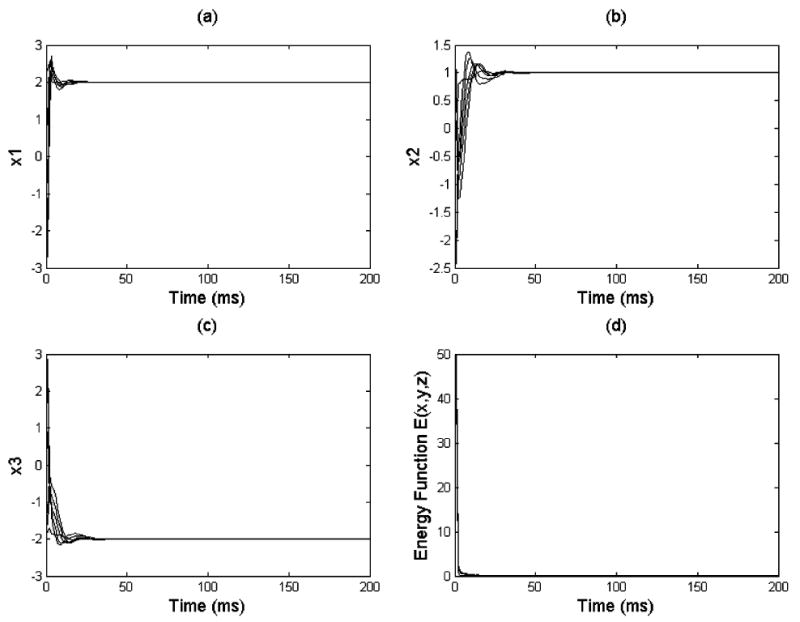
Convergence process of the CLADNN for solving ill-conditioned problem 2. (a) Convergence process of x₁ under different initial values. (b) Convergence process of x₂ under different initial values. (c) Convergence process of x₃ under different initial values. (d) Convergence process of energy function x₄ under different initial values.

$$E(\mathbf{x},\mathbf{y},\mathbf{z})={\Vert \mathbf{Cz}\mathbf{-}{\mathbf{A}}^T{P}_{\mathrm{\Omega }}(\mathbf{y}+\mathbf{Ax}\mathbf{-}\mathbf{b})\Vert }_2^2+{\Vert {\mathbf{C}}^T\mathbf{x}\mathbf{-}\mathbf{d}\Vert }_2^2.$$

C. Experiment 3: Nonlinear Curve-Fitting Problem

Let us consider a constrained nonlinear LAD curve-fitting problem: Find the parameters of the combination of polynomial and exponential function, y(x) = a₄x³ + a₃x² + a₂x + a₁e^x/2 + a₀, which fits the data given in Table I, simultaneously satisfying the constraints y(4.5) = −1.83 and y(5) ≤ −3. We can formulate this problem into the LAD problem with constraints of equality and inequality in form

TABLE I.

Nonlinear Fitting Data for Experiment 3

x	0	0.5	1	1.5	2	2.5	3	3.5	4	4.5	5
y	-9	-8	-7.6	-9	-7.1	-6.4	-3	-3.8	-2.4	-1.8	-3.1

$$\{\begin{array}{ll}\mathrm{Minimize}& {\Vert \mathbf{Ax}-\mathbf{b}\Vert }_1\\ \mathrm{Subject\; to}& {\mathbf{C}}^T\mathbf{x}=\mathbf{d},{\mathbf{E}}^T\mathbf{x}\le \mathbf{f}.\end{array}$$ (31)

where the equation shown at the top of the next page, holds. We use the MATLAB SIMULINK simulator as shown in Fig. 2(a) to implement the CLADNN for solving the problem in (31), by replacing C and d in the network with G and h, respectively, where G = [C −C E] and h = [d −d f]^T, and adding a limiter to implement the operation: E₁ = max(0, G^T x − h). By inputting the previous parameters into the simulator and starting simulations for 100 times with 100 different initial values, we get the solution converge curves as shown in Fig. 4(a), indicating that the solution is x = [1.01 −0.46 10.09 −14.28 5.28]^T and it is independent of initial values. Replacing a₄, a₃, a₂, a₁, and a₀ with this solution in y(x) = a₄x³ + a₃x² + a₂x + a₁e^x/2 + a₀, we can draw the curve fitting as shown in Fig. 4(b) (solid line). By changing L₁-norm into L₂-norm in (31) and invoking MATLAB optimization routine, namely lsqlin, we obtain the constrained LS curve fitting, as shown in Fig. 4(b) (dashed–dotted line). It has been shown that due to outliers at points (1.5, −9) and (3, −3), LS fitting performance is degenerated severely, but the CLADNN fitting is not affected, indicating that CLADNN has a more robust performance than the constrained LS optimization.

Fig. 4.

Solving a nonlinear-fitting problem using the CLADNN. (a) Solution convergence process for solving problem 3 (nonlinear fitting). (b) Comparison of the two nonlinear-fitting methods between the CLADNN (solid line) and the constrained LS (L₂-norm) optimization (dashed–dotted line).

$$\begin{array}{ll}\mathbf{A}& ={\left[\begin{array}{ccccccccccc}0& 0.125& 1& 3.375& 8& 15.625& 27& 42.875& 64& 91.125& 125\\ 0& 0.25& 1& 2.25& 4& 6.25& 9& 12.25& 16& 20.25& 25\\ 0& 0.5& 1& 1.5& 2& 2.5& 3& 3.5& 4& 4.5& 5\\ 1& 1.284& 1.649& 2.117& 2.718& 3.49& 4.48& 5.75& 7.389& 9.488& 12.183\\ 1& 1& 1& 1& 1& 1& 1& 1& 1& 1& 1\end{array}\right]}^T\\ \mathbf{b}& ={\left[\begin{array}{ccccccccccc}\mathbf{-}9& \mathbf{-}8& \mathbf{-}7.6& \mathbf{-}9& \mathbf{-}7.1& \mathbf{-}6.4& \mathbf{-}3& \mathbf{-}3.8& \mathbf{-}2.4& \mathbf{-}1.8& \mathbf{-}3.1\end{array}\right]}^T\begin{array}{cc}d=\mathbf{-}1.83& f=\mathbf{-}3\end{array}\\ \mathbf{C}& ={\left[\begin{array}{ccccc}91.125& 20.25& 4.5& 9.488& 1\end{array}\right]}^T\\ \mathbf{E}& ={\left[\begin{array}{ccccc}125& 25& 5& 12.183& 1\end{array}\right]}^T\end{array}$$

and

$$\mathbf{x}={\left[\begin{array}{lllll}{a}_4& a_3& a_2& a_1& a_0\end{array}\right]}^T$$

V. Conclusion

A new NN, namely, CLADNN, to solve the constrained LAD problems has been proposed in this paper. It has been mathematically shown that the proposed CLADNN is Lyaponov stable and it is able to globally converge to the exact solution of a given constrained LAD problem if it does exist. We have conducted three numerical simulations using the MATLAB SIMULINK simulator of the CLADNN. It has been demonstrated that the CLADNN can be used to solve linear and nonlinear curve-fitting problems. In addition, the CLADNN is able to give an exact solution to some ill-conditioned unconstrained LAD problems if prior information is available serving as a certain constraint. This is a promising feature for real-world applications where the problems are often ill-conditioned, but some prior information may be available for the solution, for example, in typical spectra quantification of magnetic resonance spectroscopy (MRS) where the frequencies of some metabolisms may be known. As illustrated in solving the nonlinear curve-fitting problem, compared with conventional LS (L₂-norm) optimization, the CLADNN is more robust in spiky noise environment, which is of great application potentials in modeling brain imaging data, such as functional magnetic resonance imaging (fMRI) and diffusion tensor imaging (DTI) data since the scanning process often suffers severely from sudden movements of the head, especially, when the subjects are children, which make the final data contain a lot of spiky noise or outliers. Therefore, the applications of the proposed CLADNN to real-world problem deserve further exploration.

Biographies

Zhishun Wang (M’99–SM’99) received the Ph.D. degree in signal processing from Southeast University, Nanjing, China, in 1997.

Currently, he is an Assistant Professor in Brain Imaging at the Department of Psychiatry, Columbia University, New York, NY. He is also a Research Scientist at the New York State Psychiatry Institute, New York. He has been extensively working on brain imaging and its application to the research of human cognitive process and childhood psychiatry with an emphasis on signal processing of functional magnetic resonance imaging (fMRI). His research interests include functional and structural MRI, multidimensional signal/image processing, neural networks, chaos and fractal in the brain and the gut, independent component analysis, wavelet, and functional and effective brain connectivity.

Dr. Wang received the “Excellent Doctoral Thesis Award in Year 2000” from the Academic Committee of the State Council of China for his Ph.D. dissertation.

Bradley S. Peterson received the M.D. degree from the University of Wisconsin—Madison in 1987.

Currently, he is the Suzanne Crosby Murphy Professor in Pediatric Neuropsychiatry and Director of MRI Research at the Department of Psychiatry, Columbia University, New York, and New York State Psychiatric Institute, New York. He trained in general psychiatry at Massachusetts General Hospital and Harvard University, in child psychiatry at the Child Study Center of Yale University, and in MRI methodologies at Yale University. His research interests include neuropsychiatry and multimodality neuroimaging of childhood psychiatry.

References

- 1.Cichocki A, Unbehauen R. Neural networks for solving systems of linear equations—Part II: Minimax and least absolute value problems. IEEE Trans Circuit Syst. 1992 Sep;CAS-39(9):619–633. [Google Scholar]
- 2.Cichocki A, Unbehauen R. Neural Networks for Computing, Optimization and Signal Processing. Stuttgart, Germany: Teubner-Wiley; 1993. [Google Scholar]
- 3.Zala CA, Barrodale I, Kennedy JS. High-resolution signal and noise field estimation using the L1 (least absolute values) norm. IEEE J Ocean Eng. 1987 Jan;OE-12(1):253–264. [Google Scholar]
- 4.Barrodale I, Zala CA. L1 and L∞ curve fitting and linear programming algorithms and applications. In: Mohamed JL, Walsh JE, editors. Numerical Algorithms. ch. 11. Oxford, U.K.: Oxford Univ. Press; 1986. pp. 220–238. [Google Scholar]
- 5.Bandler JW, Kellerman W, Madsen K. A nonlinear L1 optimization algorithm for design, modeling, and diagnosis of networks. IEEE Trans Circuits Syst. 1987 Feb;CAS-34(1):174–181. [Google Scholar]
- 6.Abdelmalek NN, Ostu N. Restoration of images with missing high-frequency components by minimizing the L1 norm of the solution vector. Appl Opt. 1986;24:1415–1420. doi: 10.1364/ao.24.001415. [DOI] [PubMed] [Google Scholar]
- 7.Bloomfield P, Steiger WL. Least Absolute Deviations: Theory Applications and Algorithms. Boston, MA: Brikhäuser; 1983. [Google Scholar]
- 8.Ward RK. An on-line adaptation for discrete L1 linear estimation. IEEE Trans Autom Control. 1984 Jan;AC-29(1):67–71. [Google Scholar]
- 9.Ruzinsky SA, Olsen ET. L1 and L∞ minimization via a variant of Karmarkar’s algorithm. IEEE Trans Acoust Speech Signal Process. 1989 Feb;37(2):245–253. [Google Scholar]
- 10.Levy S, Walker C, Ulrych TJ, Fullagar PK. A linear programming approach to the estimation of the power spectra of harmonic processes. IEEE Trans Acoust Speech Signal Process. 1982 Aug;ASSP-30(4):675–679. [Google Scholar]
- 11.Wang ZS, Cheung JY, Xia YS, Chen J. Neural implementation of unconstrained minimum L1-norm optimization—Least absolute deviation model and its application to time delay estimation. IEEE Trans Circuits Syst II Analog Digit Signal Process. 2000 Nov;47(11):1214–1226. [Google Scholar]
- 12.Wang ZS, He Z, Chen J. Robust time delay estimation of bioelectric signals. IEEE Trans Biomed Eng. 2005 Mar;52(3):454–462. doi: 10.1109/TBME.2004.843287. [DOI] [PubMed] [Google Scholar]
- 13.Wang ZS, Cheung JY, Xia YS, Chen J. Minimum fuel neural networks and their applications to overcomplete signal representations. IEEE Trans Circuits Syst I Fundam Theory Appl. 2000 Aug;47(8):1146–1159. [Google Scholar]
- 14.Hopfield JJ, Tank DW. Neural computation of decisions in optimization problems. Biol Cybern. 1985;52:141–152. doi: 10.1007/BF00339943. [DOI] [PubMed] [Google Scholar]
- 15.Tank DW, Hopdield JJ. Simple neural optimization networks: An A/D converter, signal decision circuit, and a linear programming circuit. IEEE Trans Circuit Syst. 1986 May;CAS-33(5):533–541. [Google Scholar]
- 16.Kennedy MP, Chua LO. Neural networks for nonlinear programming. IEEE Trans Circuit Syst. 1988 May;CAS-35(5):554–562. [Google Scholar]
- 17.Maa CY, Shanblatt MA. A two-phase optimization neural network. IEEE Trans Neural Netw. 1992 Nov;3(6):1003–1009. doi: 10.1109/72.165602. [DOI] [PubMed] [Google Scholar]
- 18.Sudharsannan S, Sundareshan M. Exponential stability and a systematic synthesis of a neural network for quadratic minimization. Neural Netw. 1991;4:599–613. [Google Scholar]
- 19.Wu X, Xia Y, Li J, Chen WK. A high performance neural network for solving linear and quadratic programming problems. IEEE Trans Neural Netw. 1996 May;7(3):525–529. doi: 10.1109/72.501722. [DOI] [PubMed] [Google Scholar]
- 20.Xia YS. A new neural network for solving linear programming problems and its application. IEEE Trans Neural Netw. 1996 Mar;7(2):525–529. doi: 10.1109/72.485686. [DOI] [PubMed] [Google Scholar]
- 21.Xia YS, Wang J. A general methodology for designing globally convergent optimization neural networks. IEEE Trans Neural Netw. 1998 Nov;9(6):1331–1343. doi: 10.1109/72.728383. [DOI] [PubMed] [Google Scholar]
- 22.Rodriquez-Vazquez A, Dominquez-Castro R, Rueda A, Huertas JL, Sanchez-Sinencio E. Nonlinear switched-capacitor neural networks for optimization problems. IEEE Trans Circuits Syst. 1990 Mar;37(3):384–398. [Google Scholar]
- 23.Huang DS. A constructive approach for finding arbitrary roots of polynomials by neural networks. IEEE Trans Neural Netw. 2004 Mar;15(2):487–491. doi: 10.1109/TNN.2004.824424. [DOI] [PubMed] [Google Scholar]
- 24.Huang DS, Ip HHS, Chi Z. A neural root finder of polynomials based on root moments. Neural Comput. 2004;16:1721–1762. [Google Scholar]
- 25.Miller RK, Michel AN. Ordinary Differential Equations. New York: Academic; 1982. [Google Scholar]
- 26.Luenberger DG. Introduction to Linear and Nonlinear Programming. Reading, MA: Addison-Wesley; 1973. [Google Scholar]
- 27.LaSalle J. Stability theory for ordinary differential equations. J Differ Equ. 1968;4:57–65. [Google Scholar]
- 28.LaSalle J, Lefschetz S. Stability by Lyapunov’s Direct Method with Applications. New York: Academic; 1961. [Google Scholar]
- 29.LaSalle J. The Stability of Dynamical Systems. Philadelphia, PA: SIAM; 1976. [Google Scholar]
- 30.Kinderlehrer D, Stampcchia G. An Introduction to Variational Inequalities and Their Applications. New York: Academic; 1980. [Google Scholar]
- 31.Tsividis Y, Anastassiou D. Switched-capacitor neural networks. Electron Lett. 1987;23:958–959. [Google Scholar]
- 32.Cichocki A, Ramirez-Angulo J, Unbehauen R. Architectures for analog VLSI implementation of neural networks for solving linear equations with inequality contraints. Proc IEEE Int Symp Circuits Syst. 1992 May;3:1529–1532. [Google Scholar]
- 33.Cichocki A, Unbehauen R. Switched-capacitor neural networks of linear equations and related problems. IEEE Trans Circuit Syst. 1992 Feb;39(2):124–138. [Google Scholar]