Modelling molecular interaction pathways using a two-stage identification algorithm

Abstract

In systems biology, molecular interactions are typically modelled using white-box methods, usually based on mass action kinetics. Unfortunately, problems with dimensionality can arise when the number of molecular species in the system is very large, which makes the system modelling and behavior simulation extremely difficult or computationally too expensive. As an alternative, this paper investigates the identification of two molecular interaction pathways using a black-box approach. This type of method creates a simple linear-in-the-parameters model using regression of data, where the output of the model at any time is a function of previous system states of interest. One of the main objectives in building black-box models is to produce an optimal sparse nonlinear one to effectively represent the system behavior. In this paper, it is achieved by applying an efficient iterative approach, where the terms in the regression model are selected and refined using a forward and backward subset selection algorithm. The method is applied to model identification for the MAPK signal transduction pathway and the Brusselator using noisy data of different sizes. Simulation results confirm the efficacy of the black-box modelling method which offers an alternative to the computationally expensive conventional approach.

Introduction

The phenotypic behavior of living organisms is determined by the underlying and highly complex interactions of molecules, for example proteins, DNA, RNA or other biochemical substances (Kitano 2002). These interactions can occur at an extremely fast rate and therefore the overall dynamics of the cell or higher organism is highly nonlinear. One of the challenges of systems biology is to utilize proven techniques that have been developed in other areas, such as control engineering, and apply these to biological systems in order to try to gain a better understanding of the function and behaviour of the underlying molecular processes (Wolkenhauer et al. 2005; Wellstead 2007).

This paper investigates two such processes that have been widely studied in the literature: the mitogen-activated protein kinase (MAPK) cascade (Gormley et al. 2007; Sasagawa et al. 2005; Huang and Ferrell 1996; Kholodenko 2000) and a biological oscillator known as the Brusselator (Karafyllis et al. 1997; Peng and Wang 2005; Wang et al. 2002; Zimmerman 2006). The MAPK cascade can be found in all eukaryotic cells and is an important signal transduction pathway that helps to activate several transcription factors involved in the regulation of cell cycle activity (Widmann et al. 1999). The Brusselator is a simplified model of biochemical oscillations; a behaviour that is the basis for much of the dynamic behaviour found in many cellular systems. For example, the regulation of enzyme activity produces metabolic oscillations, circadian rhythms originate from the regulation of gene expression, and oscillations in intracellular calcium levels are responsible for the control of cell receptor activity which in turn is responsible for intercellular signalling (Goldbeter 2002). Therefore, identifying the key features and dynamics in these types of molecular processes is important for understanding system behaviour and also for possible regulatory control of biological systems.

Throughout the systems biology literature, the most common approach to representing these molecular interactions and signalling pathways is by ordinary/partial differential equations (Levchenko et al. 2000; Chen et al 2004; Markevich et al. 2007). Such equations describe concentration levels of the individual molecular species in the pathway over time. In control engineering, this is commonly known as white-box modelling as the models have been derived from chemical rate equations of the underlying biological process to provide a complete picture of the system at any time. Such models are perfectly feasible when the number of molecular species in the pathway is relatively small (such as in the cases investigated here). However, in other biological systems the number of species interactions can become incredibly large, resulting in the model becoming too complex to analyse and even impossible to solve. The work described here therefore takes a different approach by adopting simplified black-box identification of these biological systems using a linear-in-the-parameters model. This class of nonlinear model comprises of a linear combination of some model terms or basis functions, that are a function of past system states of interest, and has been used to model a wide range of nonlinear dynamic systems in the literature. Some examples include the polynomial nonlinear AutoRegressive model with eXogenous inputs (polynomial NARX), neurofuzzy networks, and radial basis function (RBF) networks (Chen et al. 1989; Haber and Unbehauen 1990; Sjberg et al. 1995; Li et al. 2005, 2006; Peng et al. 2006). It has been shown that linear-in-the-parameters models have broad approximation capabilities and have been widely used in modelling and control of complex nonlinear engineering systems (Chen et al. 1989; Harris et al. 2002; Zhu and Billings 1996; Li et al. 2004; Huang et al. 2005; Hunt et al. 1992).

When building a linear-in-the-parameters model, a major problem is that a very large pool of candidate model terms has to be considered initially (Mao and Billings 1997; Li et al. 2005; Haber and Unbehauen 1990), from which a useful and simplified model is then generated based on the parsimonious principle (Ljung 1987; Söderström and Stoica 1989), of selecting the smallest possible model, in terms of size, which explains the data. In the linear regression field, this problem is referred to as the subset selection (Draper and Smith 1981; Hastie et al. 2001; Lawson and Hanson 1974; Miller 1990; Li et al. 2006). However, in modelling nonlinear dynamic systems, the size of the term pool can be so huge (Mao and Billings 1997) that to select an optimal subset is computationally too expensive. For example, (Mao and Billings 1997) pointed out that exhaustive search of the optimal model with 20 possible model terms involves 2.43 × 10¹⁸ search paths—the so-called curse of dimensionality.

Among various subset approaches, the forward methods are among the most effective for model building where a very large term pool has to be considered. In particular, the orthogonal least squares (OLS) method (Chen et al. 1989; Chen and Wigger 1995; Zhu and Billings 1996), which performs the forward stepwise model selection using modified Gram–Schmidt (MGS) orthogonalization, is the most popular one. In forward model selection, significant terms are selected one-by-one, and the net decrease in the cost function due to each newly selected term can be computed without explicitly solving the least-squares. Thus the computational complexity is significantly reduced and the dimensionality problem can be effectively relieved. To further improve the computational efficiency and numerical stability, other fast algorithms have been proposed (Li et al. 2005; Chen and Wigger 1995; Korenberg 1988).

Despite the great efficiency of forward stepwise methods in model selection, the major disadvantage is that the model obtained is not optimal (Sherstinsky and Picard 1996). To overcome this problem, the orthogonal estimation algorithm has been augmented with genetic search procedures to search the optimal model (Mao and Billings 1997). However, it is well known that genetic algorithms suffer from slow and premature convergence (Andre et al. 2001; Peng et al. 2004). Given the fact that the search for the optimal model is a mixed integer problem and that numerous local minima exist, there is no guarantee that the global optimum can be produced in practice through a genetic search. Moreover, the computational complexity is usually extremely high, and it is also impossible to analyse this due to the stochastic sampling nature of genetic search.

In this paper, an iterative subset selection approach is used for identification of the nonlinear dynamics of molecular interactions that underly many biological systems. The model terms are selected and refined within one analytic framework, leading to improved model compactness over forward subset selection methods. It will be shown that the proposed method can capture the inherent dynamics of these systems using only sparse input–output data of system states, where the sets are of varying size. It will be demonstrated that the method is of sufficient accuracy, even considering system noise, to offer a simple alternative to the more computationally expensive white-box approach.

This paper is organised as follows. The next section describes the main method used to select the optimal model structure. Following that, the two biological systems to be investigated are introduced. The iterative subset selection method is then applied to modelling simulations of these molecular processes using a polynomial NARX structure. Finally some conclusions are drawn.

The modelling method

The method applied to modelling the biological systems in this paper is a polynomial NARX model. This type of model uses regression of system input–output data to create a model structure and has been applied to modelling many types of conventional nonlinear systems throughout the control engineering literature. The ability of these models to approximate any nonlinear function to arbitrary accuracy is well known (Ljung 1987). They provide a method of mapping input states to system output, where the internal structure of the target system is usually not considered. These are relatively simple linear-in-the-parameters models, where the output at any time is a linear combination of previous input/output states of the system. For readers less familiar with this type of approach, the following subsection provides a brief introduction to the technique.

Introduction to polynomial NARX models

A general nonlinear dynamic system can be represented as:

1

where the output of the system y(t) at any time is a function of previous output and input states u(t) plus some unknown noise variation where n_u and n_y are the maximal input/output lags, x(t) is the model ‘input’ vector, and f(·) is some unknown (usually nonlinear) function.

Now suppose the systems to be investigated are represented by a polynomial NARX model, which is a linear-in-the-parameters model of the form:

2

where φ is the regression matrix which contains M candidate model terms and θ is the corresponding vector of model parameters to be estimated.

The regression matrix φ is constructed from a polynomial expansion of previous input and output states of the target system. The main steps taken to construct it are as follows:

1. First perturb the target system to obtain a set of input–output data evenly sampled over a period of time.

2. Now taking the input u(t) and output y(t) vectors of N samples each, create new data vectors by delaying u(t) and y(t) by a number of time points to create the model input vector x(t). So for example a system lag of 3 would create a model input vector of:

   3

3. Next perform a polynomial expansion of the model input vector x(t) to create the full regression matrix φ. So for a polynomial expansion of 3, φ would be a N × M matrix containing M = 14 column vectors of linear and nonlinear candidate terms of up to 2nd order.

Now the problem is to select the best n regressor terms p₁,…,p_n ∈ [φ₁,…,φ_M] so that the sum squared error (SSE) between the target system and model output is minimised:

4

Through minimising the cost function, the model parameters are also estimated and the significance of each term in the regression matrix towards the true system can be established. Terms that are unrelated to the true system will be found to have an insignificant contribution to minimising the cost function and hence, the most important regressor terms can be selected to be included in the model.

Obviously, when building a model, both the order of expansion and number of delays selected for the input vector will affect the performance. Increasing these parameters means that the subset selection algorithm will be more likely to converge upon the optimal model, however, this will also increase the solution space as M tends towards infinity and therefore the computational complexity of finding the solution becomes too high.

Implementation example

To illustrate the basic concept proposed in the paper, consider the following true system which is unknown to the modeler:

5

Now, if a NARX model is created with five delays on the model input vector with a polynomial expansion of order 2, the full model can be constructed as:

6

Now comparing this to the true system shows that only linear terms are required in this case, so ideally the model subset selection algorithm will only select these terms when performing the regression, while ignoring the insignificant nonlinear terms.

However, suppose a set of observations (samples) has been obtained from the true system, based on which a run of the forward selection algorithm might have selected the following four terms:

7

Comparing this with the true system shows that only two of the most significant terms have been selected, even though the model may still be able to give a reasonable approximation of the system.

Now if instead we perform the forward and backward subset selection algorithm proposed in this paper, the terms selected are:

8

This algorithm has selected the most significant model terms and has therefore converged upon the optimal model structure resulting in greater transparency in the model and an improved modelling performance.

The 2-stage algorithm

The two-stage identification algorithm used to perform the subset selection is only briefly described in the following subsections. A more detailed algorithm can be found in the Appendix section.

Forward subset selection

This section briefly outlines the first stage of the identification method where the algorithm uses forward selection to generate an initial model. The model terms are chosen one-by-one from a pool of candidates so that each time the cost function is reduced by the maximum amount. This procedure is repeated until k model terms have been selected, where k is determined by the model structure selection criterion.

To begin with, consider a general nonlinear dynamic system (Chen et al. 1989; Li et al. 2005, 2006)

9

where u(t) and y(t) are the system input and output at sample time instant t, n_u and n_y are the corresponding maximal lags, x(t) represents the model ‘input’ vector, and f(·) is some unknown nonlinear function.

Now suppose in this case a polynomial NARX model is used to represent system (9), then

10

where φ_i(·), i = 1,…, M are candidate basis functions and ɛ(t) is the model residual. If a sequence of N data samples {x(t), y(t)}, t = 1,…, N is to be used for model identification, Eq. (10) can be rewritten as:

11

where with for i = 1,…, M, , and .

The model selection aims to select, say k, regressor terms, denoted as p₁,…,p_k, from all the candidates, (M is usually ≫ k), resulting in a linear-in-the-parameters model

12

which best fits the data samples such that the sum squared-error (SSE) is minimised where

13

Here is an N × k matrix composing of k columns from denotes the corresponding regression coefficient vector, and the selected regression matrix

14

If P_k is of full column-rank, the least-squares estimate of the regression coefficients in (12) is given by

15

Having selected k model terms, suppose that one more is added into the model with the corresponding regressor term p_k+1. The net reduction in the cost function due to adding this term is now given by

16

Evaluating the contribution of all remaining terms requires some redefinitions:

17

Now clearly the first k regressors in Φ (i.e. P_k) correspond to the selected k terms, while the remaining M−k terms C_M−k = [ϕ_k+1,⋯, ϕ_M] make up the candidate pool C_M−k.

Using (16) the contribution of all remaining candidate terms in Φ = {ϕ₁,…,ϕ_M} can now be calculated and the term from C_M−k which gives the maximum contribution is then selected as the (k + 1)th model term. For example, if the index j of the next most significant term is given by

18

then ϕ_j is selected as the (k + 1)th model term and re-labelled as p_k+1 = ϕ_j. The regression matrix of the selected model is then P_k+1 = [P_k p_k+1], while the candidate pool is reduced in size and becomes C_M−k−1. The remaining candidates in C_M−k−1 are re-indexed as ϕ_k+2,⋯,ϕ_M. Finally, the full regression matrix Φ changes to Φ = [P_k+1 C_M−k−1].

This forward selection is repeated until the desired number of model terms (k) has been reached, or the cost function is reduced to a given level, or a certain stop criterion has been reached, such as Akaike’s information criterion (AIC) (Akaike 1974) or the minimum description length (MDL) (Gustafsson and Hjalmarsson 1995). Once the initial model has been constructed, the model can be refined using a backward selection approach to replace insignificant model terms in the original structure.

Backward model refinement

Each iteration of the forward selection algorithm described above selects one new term and adds this to the model. The term is chosen as the one that produces the maximum reduction in the cost function. However, there is usually some correlation between the regressor terms. Therefore terms that are selected subsequently may affect the contribution of previously selected ones. In other words, while a previously selected model term may once have provided a large contribution to reducing the cost, due to a newly introduced term, its contribution can suddenly become insignificant. This inefficiency in forward subset selection methods has been explored in (Sherstinsky and Picard 1996). To overcome this a second stage is introduced whereby all the previously selected model terms are reviewed and the model is refined. Any insignificant terms are removed and/or replaced until an optimal model is achieved for a given selection criterion.

Assume an initial model with n regressor terms has been generated using forward selection. Then suppose a term, say p_i, 1 ≤ i≤ n, is to be reviewed. Its contribution to the cost (SSE) reduction ΔJ_n (p_i) needs to be compared to the individual in the pool of candidate terms offering the largest contribution to cost reduction. Denoting the maximum candidate contribution as , then the significance of a model term p_i can be checked by identifying the maximum of the contribution of all the other candidates from

19

If is said to be insignificant, and will be replaced with as the new regressor term, while p_i is returned to the candidate pool, taking the position of . Such an exchange of model terms will further reduce the SSE by , which means that the model compactness is further improved and an optimal model structure can be obtained.

The experimental results

The following sections now provide a description of the steps taken to perform the identification of two simulated biological systems using the proposed method from the previous section. The two systems investigated here are the MAPK signalling pathway and the Brusselator. In each case a brief introduction to the system is given, along with a description of the modelling process. Finally, the modelling results obtained using the two-stage algorithm are compared with the conventional forward selection approach.

The MAPK cascade

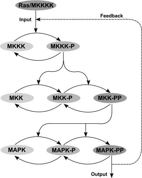
The MAPK cascade is an important intracellular signalling pathway that is involved in producing many different cellular responses, including cell growth and proliferation (Kholodenko 2000). As such, it is an important pathway that can even be implicated in cancer development when its normal signalling process malfunctions. The pathway describes the response of a cell when it detects the binding of extracellular signalling molecules to receptor proteins at the surface of the cell membrane. The binding process results in conformational changes on the part of the receptor that is below the membrane surface, which in turn triggers the activation of a cascade of intracellular signalling proteins. This is a three-tiered cascade where the kinase at each level is activated through dual phosphorylation at two amino acid sites by the activated kinase of the previous level (see Fig. 1). At the end of the cascade, the terminal signalling protein activates target proteins which alter the behaviour of the cell, for example, by regulating the expression of certain genes, by altering cell shape (by cytoskeletal proteins) or by changing cell metabolism (Alberts et al. 2002).

Fig. 1.

Kinetic pathway diagram of the MAPK cascade. The single and dual phosphorylation of each molecule is represented by the addition of a ‘-P’ and ‘-PP’ respectively to the name of the kinase, where MAPK-PP represents the output activated form of the kinase. Ras (or MKKKK) is the input protein that triggers the activation of the kinase at the top level of the cascade

Simulation of the MAPK cascade

To create a black-box model of the MAPK cascade, a set of input–output data is required to perform model estimation and validation. A simulation of the signalling pathway was performed to generate a sufficiently large data set. The mathematical model used for the simulation is based on one derived in (Kholodenko 2000) which includes the addition of negative feedback. This is an 8th order state model with a single-input and single-output (SISO). The model uses Michaelis–Menten enzyme kinetics to derive chemical rate equations for each of the pathway connections in the cascade. The rate equations are given in Tables 1 and 2. After setting the initial concentrations of each species and rate constants, the physical equations can be solved for a particular time series.

Table 1.

Kinetic rate equations for the concentrations of each of the eight types of molecule found in the MAPK cascade (Kholodenko 2000)

d[MKKK]/dt = v2−v1

d[MKKK-P]/dt = v1−v2

d[MKK]/dt = v6−v3

d[MKK-P]/dt = v3 + v5−v4−v6

d[MKK-PP]/dt = v4−v5

d[MAPK]/dt = v10−v7

d[MAPK-P]/dt = v7 + v9−v8−v10

d[MAPK-PP]/dt = v8−v9

Moiety conservation relations:

[MKKK]total = [MKKK] + [MKKK-P] = 100

[MKK]total = [MKK] + [MKK-P] + [MKK-PP] = 300

[MAPK]total = [MAPK] + [MAPK-P] + [MAPK-PP] = 300

Table 2.

Rate equations and parameters for each of the 10 reactions in the MAPK pathway diagram (Fig. 1)

Reaction	Rate equation
v1	k1  ·  [Ras0] · [MKKK]/((1 + ([MAPK-PP]/KI)n) · (K1 + [MKKK]))
v2	V2 · [MKKK-P]/(K2 + [MKKK-P])
v3	k3 · [MKKK-P] · [MKK]/(K3 + [MKK])
v4	k4 · [MKKK-P] · [MKK-P]/(K4 + [MKK-P])
v5	V5 · [MKK-PP]/(K5 + [MKK-PP])
v6	V6 · [MKK-P]/(K6 + [MKK-P])
v7	k7 · [MKK-PP] · [MAPK]/(K7 + [MAPK])
v8	k8 · [MKK-PP] · [MAPK-P]/(K8 + [MAPK-P])
v9	V9 · [MAPK-PP]/(K9 + [MAPK-PP])
v10	V10 · [MAPK-P]/(K10 + [MAPK-P])

The Michaelis–Menten constants (K_I = 9, K₁ = 10, K₂ = 8, K₃−K₁₀ = 15) and molecular concentrations are given in nM. [Ras₀] is the initial concentration of the input protein or MKKK kinase. The catalytic rate constants (k₁ = k₃ = k₄ = k₇ = k₈ = 0.025) and the maximal enzyme rates (V₂ = 0.25, V₅ = V₆ = 0.75, V₉ = V₁₀ = 0.5) are given in units of s⁻¹ and nM·s⁻¹ respectively (Kholodenko 2000)

Identification of the MAPK cascade

A data set of 800 samples was generated from the simulation of the MAPK signalling cascade. In order to simulate the effects of measurement noise, a signal of uniformly distributed random noise was generated for each time point and added to the data. The noise was at a level of 30 dB of the signal power of the original data. Finally, the data was normalised to within the range 0–1 and the corresponding statistical measures for this set can be seen in Table 3.

Table 3.

Statistics of the input–output data sets used for training and validation

	Training		Validation
	ut	yt	ut	yt
Mean	0.5255	0.4158	0.5036	0.4494
Std. deviation	0.2871	0.2882	0.2930	0.2778
Min–max	0–1	0–1	0–1	0–1

Ras corresponds to the input data vector (u_t) and MAPK-PP corresponds to the output data vector (y_t)

Ideally when performing this type of regression modelling, a large data set (typically 1,000–2,000 samples) is used to make certain that the model will capture the entire range of possible dynamics of the system. However, when dealing with biological systems the amount of data available using current experimental techniques is much smaller than this. For example a typical differential equation model in the Systems Biology literature is fitted to a set of around 30–50 data points. This could be a potential stumbling block for applying the proposed two-stage algorithm to model biological systems. However, provided the derived model is able to perform well when validated on previously unseen data, then the model can be said to be sufficiently accurate. To investigate the effect that data size has on performance, models were derived using subsets of the original 800 samples, beginning with 30 samples and gradually increasing this up to 400 samples.

In each case a nonlinear polynomial AutoRegressive model with eXogenous inputs (NARX), with polynomial order up to 3, was used to construct the regression model. The model input variables Ras (u_t) and MAPK-PP (y_t), with delays of up to 3 time steps each, were used to construct the full model set, resulting in a candidate pool of 285 terms. First the forward selection procedure was performed (using the MDL as the stop criterion) to select a subset of terms from the pool and estimate the corresponding model parameters. Then the obtained model structure was validated on a new set of 400 data points not provided to the algorithm during estimation. The process was then repeated for each set, this time using the proposed two-stage identification algorithm, to perform both forward and backward subset selection in each case. As mentioned in the previous section, the forward approach is not optimal therefore the two-stage method should obtain a more accurate model. To compare the performances, the results of training and validation for both methods on each data set are listed in Table 4.

Table 4.

MAPK training and validation results with mean squared error (MSE) between the model and target output given for different sized data sets

No. samples	Training		Validation
	Forward	Two-stage	Forward	Two-stage
30	0.0012	0.0008	0.0285	0.0199
50	0.0025	0.0015	0.0118	0.0088
100	0.0044	0.0029	0.0101	0.0037
200	0.0028	0.0022	0.0038	0.0031
400	0.0008	0.0006	0.0010	0.0008

From Table 4, it is clear that the proposed two-stage method outperformed the conventional forward selection method in terms of modelling accuracy. As expected the performance also increases, particularly under validation, as the amount of data available to the algorithm increases.

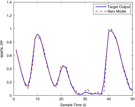
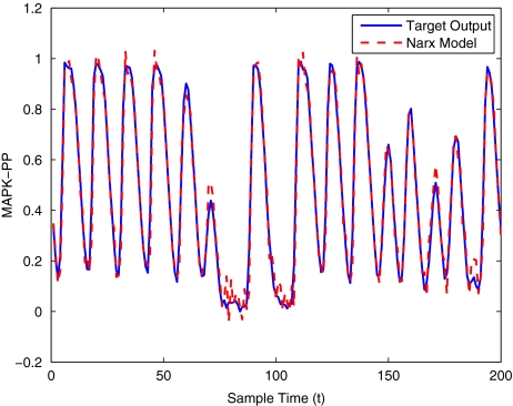
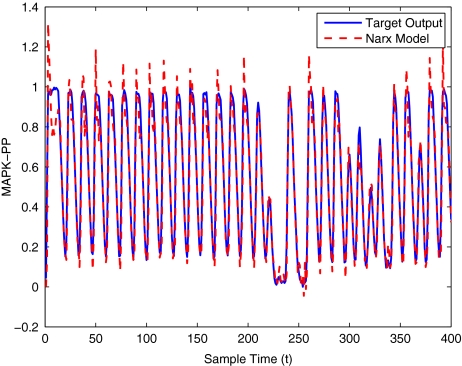
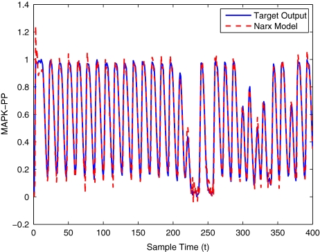
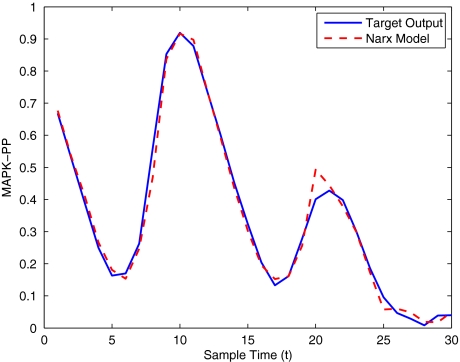
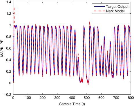
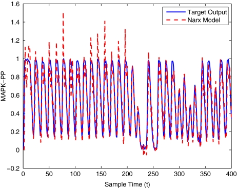
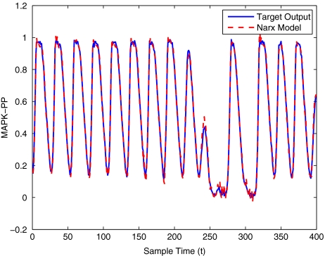
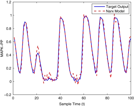
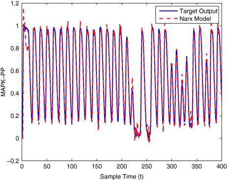
To get an indication of the ability of this method to approximate the MAPK system, Figs. 2 to 11 display the model output superimposed over the target output during the estimation and validation stages. As can be seen in Fig. 2 the polynomial NARX model can be easily fitted to the data when only 30 samples are available from the set. Unfortunately this model is then quite poor when it attempts to be validated on new unseen data in Fig. 7. As the number of samples used at the estimation stage is increased (Figs. 2–6), the performance of the models under validation also improves (Figs. 7–11). In fact even using only 100 samples for estimation (Fig. 4) the validation performance has reached an acceptable level (Fig. 9) and the NARX model can approximate the MAPK pathway to sufficient degree of accuracy.

Fig. 3.

MAPK model estimation using only 50 data points

Fig. 5.

MAPK model estimation using 200 data points

Fig. 8.

MAPK model validation using only 50 data points

Fig. 10.

MAPK model validation using 200 data points

Fig. 2.

MAPK model estimation using only 30 data points

Fig. 11.

MAPK model validation using 400 data points

Fig. 7.

MAPK model validation using only 30 data points

Fig. 6.

MAPK model estimation using 400 data points

Fig. 4.

MAPK model estimation using 100 data points

Fig. 9.

MAPK model validation using 100 data points

Taking the case of the models generated using only 100 samples as an examples, the model structure and parameters derived from both methods are given in Tables 5 and 6. Using the MDL as the stop criterion, the forward subset selection procedure produced a model structure containing only eight terms out of the entire pool of 285 candidates. When the proposed two-stage forward and backward selection method was used, a new optimal subset of eight terms was selected instead. The different subsets of terms and parameters obtained by the two approaches can be compared in Tables 5 and 6. It is obvious from looking at the tables that these model structures are very simple, consisting only of a linear combination of eight (linear/nonlinear) terms and associated parameters. Therefore as already stated in previous sections, these types of models are much simpler than their differential equation counterparts and offer a potential solution to the problem of solving complex high-dimensional systems containing a large number of variables.

Table 5.

MAPK model structure obtained from forward selection

Selection order	Term index	Terms	Param’s	SSE
1	6	yt−1	−3.5189	2.1032
2	7	yt−2	1.9256	0.8905
3	51	y2t−1	−2.5403	0.7060
4	252	y2t−1yt−2	2.0019	0.6166
5	10	yt−5	0.1762	0.5361
6	139	ut−2ut−4ut−5	−0.0910	0.5117
7	254	y2t−1yt−4	−0.4038	0.4928
8	276	y3t−3	0.1814	0.4403

The parameters P_k and regressor terms Θ_k selected are given for the case of 100 training samples. This method selected the following eight terms from the pool of 285 candidates: {6, 7, 51, 252, 10, 139, 254, 276}

Table 6.

MAPK model structure obtained from two-stage, forward and backward subset selection

Selection order	Term index	Terms	Param’s	SSE
1	132	ut−2ut−3ut−5	−0.0990	2.1193
2	56	y2t−2	2.1606	0.9038
3	51	y2t−1	−3.3213	0.7320
4	251	y3t−1	1.5365	0.3664
5	57	yt−2yt−3	−1.1189	0.3410
6	8	yt−3	0.9515	0.3163
7	7	yt−2	−3.1124	0.2984
8	6	yt−1	3.8819	0.2851

The parameters P_k and regressor terms Θ_k selected are given for the case of 100 training samples. The two-stage method selected a new set of terms: {132, 56, 51, 251, 57, 8, 7, 6}

The Brusselator

The second example describes the black-box identification of a biochemical oscillator model known as the Brusselator (Karafyllis et al. 1997). Biochemical oscillations are the underlying basis for much of the dynamic behaviour found in many cellular systems. Many biological processes that exhibit oscillatory behaviour are fundamental to life itself. A typical example of this is the cell cycle, where cell growth and division are controlled by oscillations in the levels of certain proteins and therefore by mitotic oscillations (Tyson 1991; Novak and Tyson 1997; Chen et al. 2004). Therefore, identifying the key features and dynamics in these biochemical oscillations is important for understanding the underlying dynamical behaviour and for possible regulatory control of these biological systems.

Simulation of the Brusselator

As with the previous example, a simulation of the Brusselator was performed to generate a set of input–output data for model estimation and validation. The model used for the simulation is based on the four biochemical reaction equations given below:

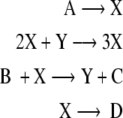This is a 6th order state model with a 2 inputs and 2 outputs. The inputs are the concentrations of molecular species A and B, and the outputs are the oscillatory species of interest X and Y. The model uses simple mass–action kinetics to derive the chemical rate equations for each of the reactions taking place in the model. From this, the rate equations for the oscillatory species of interest are derived for the Brusselator model as:

20

21

where X and Y are the outputs, A and B are input species variables and k₁, k₂, k₃ and k₄ are the rate constants. After setting the initial concentrations of A = 0.5, B = X = Y = 3.0 and C = D = 0.0 and rate constants of k₁ = k₂ = k₃ = k₄ = 1, the differential equations can be solved to generate a particular time series.

Identification of the Brusselator

From the above simulation, a data set of 800 samples was again generated to be used for model estimation and validation. As before, a uniformly distributed random noise signal was added to the data and then the sample values were normalised to within the range 0–1. Statistical measures from this new data are given in Table 7.

Table 7.

Statistics of the input–output data sets used for training and validation

	Training		Validation
	Mean	Std. deviation	Mean	Std. deviation
A	0.4906	0.2868	0.4863	0.2922
B	0.4981	0.2870	0.4911	0.2961
X	0.2014	0.1815	0.1735	0.1631
Y	0.4491	0.2103	0.4300	0.2087

A and B correspond to the input data sets (u_t) and X an Y correspond to the output data sets (y_t). All data set values were normalised to within the range 0.0–1.0

This time a polynomial NARX model of order 3, and inputs X(t−1), Y(t−1), A(t−1), B(t−1), was used to construct the full model set, resulting in a candidate pool of 454 terms. The forward subset selection procedure was performed first, and this time AIC was used as the stop criterion. For the case of modelling X(t) as the system output, 12 terms were selected from the entire candidate pool. The process was then repeated using the iterative forward and backward subset method. The different subsets of terms and parameters obtained by the two methods can be compared in Tables 8 and 9.

Table 8.

Brusselator model structure for concentration of X obtained from forward selection

Selection order	Term index	Terms	Param’s	SSE
1	73	Xt−1Yt−1	0.4519	0.2788
2	75	Xt−1Yt−3	0.1368	0.1295
3	439	Xt−3Y2t−1	−0.0669	0.1046
4	79	Xt−2Yt−2	0.0761	0.0978
5	429	Xt−2Y2t−1	0.0847	0.0926
6	425	Xt−2X2t−3	1.4923	0.0864
7	294	B2t−1Xt−2	−0.4418	0.0816
8	11	Yt−2	−0.0073	0.0750
9	419	Xt−1Y2t−3	−0.0093	0.0716
10	43	At−3Yt−1	−0.0142	0.0695
11	147	At−1Bt−3Yt−3	0.0126	0.0666
12	402	X2t−1Yt−1	−0.5576	0.0645

The parameters P_k and model terms Θ_k are given for the case of no. of training samples = 100. The forward and two-stage methods both selected a different set of terms from the pool of 454 candidates

Table 9.

Brusselator model structure for concentration of X obtained from two-stage, forward and backward subset selection

Selection order	Term index	Terms	Param’s	SSE
1	232	At−2Y2t−2	−0.0022	0.2969
2	280	At−3X2t−3	0.8045	0.1325
3	429	Xt−2Y2t−1	0.0929	0.0986
4	323	Bt−1Xt−2Yt−2	−0.1898	0.0831
5	404	X2t−1Yt−3	−0.1552	0.0739
6	43	At−3Yt−1	−0.0672	0.0703
7	402	X2t−1Yt−1	−2.1765	0.0664
8	260	At−3Bt−2Yt−2	0.0879	0.0617
9	414	Xt−1Y2t−1	−0.0299	0.0604
10	439	Xt−3Y2t−1	−0.0929	0.0594
11	75	Xt−1Yt−3	0.1809	0.0577
12	73	Xt−1Yt−1	0.8531	0.0523

The parameters P_k and model terms Θ_k are given for the case of no. of training samples = 100. The forward and two-stage methods both selected a different set of terms from the pool of 454 candidates

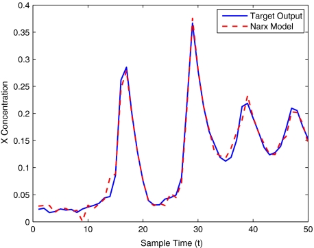
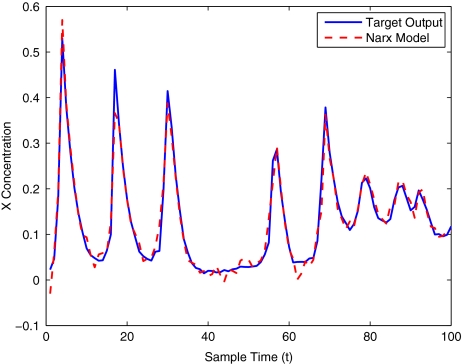
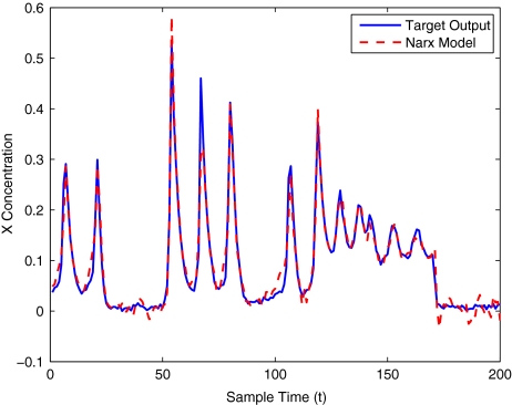
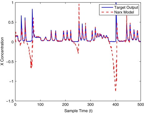
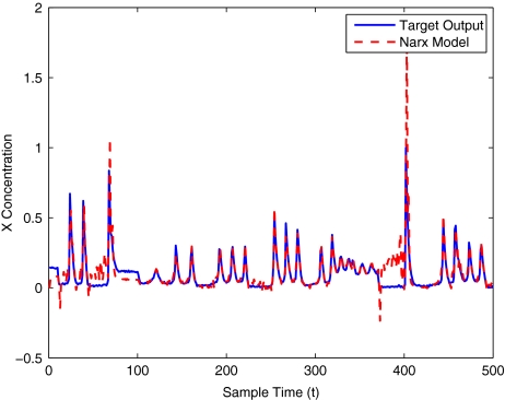
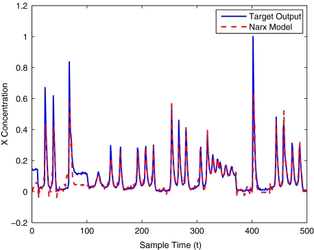
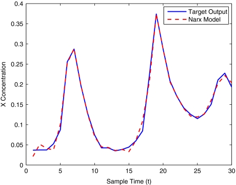
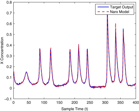
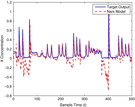
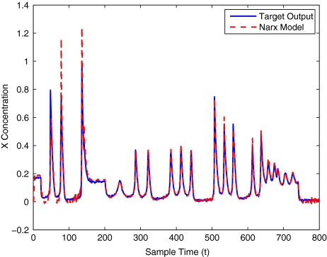
The modelling result produced by the two methods for training and validation (on different sized data sets of 30–400 samples) are listed in Table 10. Figures 12–16 show the variation in X(t) over time during the estimation stage, whereas Figs. 17–21 show this variation while attempting to validate the model over previously unseen data. These results again illustrate that the two-stage method outperforms the conventional forward approach in terms of modelling accuracy as was predicted. The figures also show that the the model begins to show a sufficient level of accuracy under validation when training has taken place on a data set of at least 100 samples.

Fig. 13.

Brusselator model estimation using only 50 data points

Fig. 14.

Brusselator model estimation using 100 data points

Fig. 15.

Brusselator model estimation using 200 data points

Fig. 18.

Brusselator model validation using only 50 data points

Fig. 19.

Brusselator model validation using 100 data points

Fig. 20.

Brusselator model validation using 200 data points

Table 10.

Brusselator training and validation results with mean squared error (MSE) between the model and target output given for different sized data sets

No. samples	Training		Validation
	Forward	Two-stage	Forward	Two-stage
30	0.0002	0.0001	0.2969	0.2311
50	0.0002	0.0001	0.0548	0.0497
100	0.0006	0.0005	0.0083	0.0046
200	0.0005	0.0004	0.0072	0.0036
400	0.0001	0.0001	0.0022	0.0010

Fig. 12.

Brusselator model estimation using only 30 data points

Fig. 16.

Brusselator model estimation using 400 data points

Fig. 17.

Brusselator model validation using only 30 data points

Fig. 21.

Brusselator model validation using 400 data points

Discussion

The work described in this paper has investigated the black-box identification of two well known nonlinear molecular interaction pathways that have traditionally been modelled using white-box methods. A two-stage approach has been used to obtain an optimal nonlinear model effectively and efficiently, where the model terms are selected and refined using a forward and backward subset selection algorithm. The simulation experiments carried out to model the Brusselator and the MAPK signalling pathway have confirmed the efficacy of the proposed algorithm. One of the main contributions of this paper has been to show that, instead of white-box modelling approaches which have been widely used in systems biology research, black box methods offer an alternative for capturing the essential behavior and dynamics of the biological processes using a simplified model structure. This enables the identification and analysis of large-scale biological systems using a relatively small set of simple models, based on which the design of control strategies may become possible. Future work will include using physically related basis functions to build up nonlinear models from the underlying biological system, improving the model transparency and interpretability.

Appendix

The two-stage identification algorithm used to perform the subset selection is outlined in the following sections of this appendix.

Problem statement and preliminaries

Consider a general nonlinear dynamic system (Chen et al. 1989; Li et al. 2005, 2006)

22

where u(t) and y(t) are the system input and output variables at time instant t, n_u and n_y are the corresponding maximal lags, x(t) represents the model ‘input’ vector, and f(·) is some unknown nonlinear function.

Suppose a nonlinear polynomial NARX model is used to represent the system (22):

23

where φ_i (·), i = 1,…, M are all candidate basis functions, and ɛ is the model residual sequence. And N data samples {x(t), y(t)}, t = 1,…, N are used for model identification. Equation (23) is then formulated as:

24

where with for and .

The model selection aims to select, say n, regressor terms, denoted as p₁,…,p_n, from all the candidates, (M is usually a very large number in nonlinear system identification), resulting in the linear-in-the-parameters model of the form

25

which best fits the data samples in the sense of least-squares, i.e. the sum squared-errors (SSE) is minimised

26

where is an N × n matrix composing of n columns from denotes the corresponding regression coefficient vector, and the selected regression matrix

27

If the selected regression matrix P_n is of full column-rank, the least-squares estimation of the regression coefficients in (25) is given by

28

Theoretically, each subset of n terms out of the M candidates forms a candidate model, and there are M!/(n!/(M−n)!) possible combinations. Obviously, to obtain the optimal subset is computationally very expensive or impossible if M is a very large number, and part of this is also referred to as the curse of dimensionality. To overcome the difficulty, an iterative subset selection method will be proposed in the following.

The main objective of the proposed method is to iteratively select and refine the model. Firstly, the method performs forward subset selection where the model terms are selected one by one with the cost function being maximally reduced each time. Once a certain model structure selection criterion is satisfied, e.g. the AIC (Akaike 1974) or MDL (Gustafsson and Hjalmarsson 1995), or the maximal reduction of the error for adding a new term is below certain threshold, then the second stage backward model refinement is performed. At the second stage, the model structure is further refined by removing all insignificant terms from the model, given that the model selection criterion is satisfied, leading to further improved model compactness and performance.

Forward subset selection

The core idea of the forward subset selection is to select the model terms one by one from a pool of candidates, each time the reduction of the cost function is maximized. This procedure is iterated until n model terms are selected (n is determined by a certain model structure selection criterion). The major objective in this subsection is to propose a fast algorithm to select the model terms.

To begin with, suppose k model terms have been selected, producing the following regression matrix

29

The corresponding cost function is given by

30

If P_k is of full column rank, then (P^T_kP_k) in (30) is symmetric and positive definite. And the optimal estimation of the coefficient is given by

31

Define

32

then, applying Cholesky decomposition to W gives

33

where D = diag(d₁, …,d_k) is a diagonal matrix and is a unity upper triangular matrix. Define

34

According to (33), it can be derived that

35

Define

36

and

37

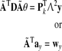
Then left-multiplying the both sides of (31) with W, and substituting (33), gives

38

a_y in (38) could be computed as

39

Then

40

Now, suppose that one more term is added into the model with the corresponding regressor term p_k+1, the cost function becomes

41

where P_k+1 = [P_k p_k+1].

Then, the net reduction of the cost function due to adding one more model term is given by

42

where a_k+1,y, a_k+1,k+1 are computed using (35) and (39) as k increases by 1.

According to (42) the selection of next model term is formulated as

43

where {ϕ₁,…,ϕ_M} is the candidate node pool.

According to (43), the contribution of all remaining candidate terms in Φ = {ϕ₁,…,ϕ_M} need to be calculated using (42). To achieve this, the dimension of A, a_y defined above will be augmented to store the information of all remaining candidate terms in Φ. To achieve this, re-define

44

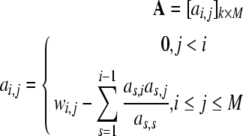
Based on (35), A is re-defined as

45

where

46

Based on (34), is re-defined as

47

and vector a_y is re-defined as

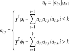48

In addition, one more M × 1 vector b is defined as

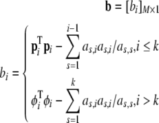49

Thus, the contribution of each of the candidates in C_M−k to the cost function can be computed as follows

50

and the one from C_M−k which gives the maximum contribution is then selected as the (k + 1)th model term.

The main body of this subsection has provided a framework to iteratively select the model terms one by one from a pool of candidates. This forward selection procedure will be terminated once the desired number (say n) of model terms have been reached or the cost function is reduced to a given level (Chen and Billings 1992), or some information criterion such as Akaike’s information criterion (AIC) begins to increase (Akaike 1974). Once an initial model has been constructed, in the following subsection, a backward approach will be proposed to refine the model to improve the model compactness and performance.

Backward model refinement

The above forward algorithm selects one regressor at a time, which maximizes the reduction of error subject to the constraint that all previously selected regressors are fixed. However, the regressors are generally correlated, later introduced regressors may affect the contribution of previously selected regressors. Therefore, the previously selected regressors may become insignificant due to the later introduced regressors. This inefficiency of forward subset selection methods have been explored in (Sherstinsky and Picard 1996). In the backward model refinement, all the previously selected model terms will be reviewed, and the model will be refined. Any insignificant terms will be removed and/or replaced, given that the model selection criterion is satisfied.

Suppose a regressor term (from a model of size n), say p_i, 1 ≤ i  ≤ n, is to be reviewed. Its contribution to the error (SSE) reduction ΔJ_n (p_i) needs to be compared with that of the one in the pool of candidate terms that can give the maximum contribution among the candidate pool. Denote the maximum candidate contribution as . If is said to be insignificant, and will be replaced with and p_i will be put back into the candidate pool. This exchange of model terms will further reduce the error (SSE) by , which means that the model compactness is further improved.

To review the model terms as explained above, the contributions for p_i and all the candidates need to be computed. To achieve efficient computation, matrices and vectors , and b, which are defined and used to compute the contributions of a regressor term in the model and in the candidate pool, have to be updated. The algorithm to update these quantities can be derived based on their definitions and follows the same procedures outlined in the forward selection algorithm, therefore will not repeated. The detailed mathematical framework can be found in (Li et al. 2006).

References

- Akaike H (1974) New look at the statistical model identification. IEEE Trans Automat Control AC-19(6):716–723
- Alberts B, Johnson A, Lewis J, Raff M, Roberts K, Walter P (2002) Molecular biology of the cell, 4th edn. Garland Science
- Andre J, Siarry P, Dognon T (2001) An improvement of the standard genetic algorithm fighting premature convergence in continuous optimization. Adv Eng Softw 32:49–60 [DOI]
- Chen S, Billings SA (1992) Neural network for nonlinear dynamic system modelling and identification. Int J Control 56:319–346 [DOI]
- Chen S, Wigger J (1995) Fast orthogonal least squares algorithm for efficient subset model selection. IEEE Trans Signal Process 43(7):1713–1715 [DOI]
- Chen S, Billings SA, Luo W (1989) Orthogonal least squares methods and their application to non-linear system identification. Int J Control 50(5):1873–1896 [DOI]
- Chen KC, Calzone L, Csikasz-Nagy A, Cross FR, Novak B, Tyson JJ (2004) Integrative analysis of cell cycle control in budding yeast. Mol Biol Cell 15:3841–3862 [DOI] [PMC free article] [PubMed]
- Draper NR, H Smith J (1981) Applied regression analysis, 2nd edn. Wiley, USA
- Goldbeter A (2002) Computational approaches to cellular rhythms. Nature 420:238–245 [DOI] [PubMed]
- Gormley P, Li K, Irwin GW (2007) Modelling the mapk signalling pathway using a two-stage identification algorithm. In: Proceedings of the international conference on life system modelling and simulation, Shanghai, China, pp 480–491
- Gustafsson F, Hjalmarsson H (1995) Twenty-one ml estimators for model selection. Automatica 31(10):1377–1392 [DOI]
- Haber R, Unbehauen H (1990) Structure identification of nonlinear dynamic systems—a survey on input/output approaches. Automatica 26:651–667 [DOI]
- Harris CJ, Hong X, Gan Q (2002) Adaptive modeling, estimation and fusion from data: a neurofuzzy approach. Springer-Verlag
- Hastie T, Tibshirani R, Friedman J (2001) The elements of statistical learning—data mining, inference and prediction. Springer-Verlag, New York
- Huang CF, Ferrell JE (1996) Ultrasensitivity in the mitogen-activated protein kinase cascade. Proc Natl Acad Sci 93:10,078–10,083 [DOI] [PMC free article] [PubMed]
- Huang GB, Saratchandran P, Sundararajan N (2005) A generalized growing and pruning rbf (ggap-rbf) neural network for function approximation. IEEE Trans Neural Netw 16:57–67 [DOI] [PubMed]
- Hunt KJ, Sbarbaro D, Zbikowski R, Gawthrop PJ (1992) Neural networks for control system—a survey. Automatica 28(3):1083–1112 [DOI]
- Karafyllis I, Christofides PD, Daoutidis P (1997) Dynamical analysis of a reaction–diffusion system with Brusselator kinetics under feedback control. In: Proceedings of the American control conference, pp 2213–2217
- Kholodenko BN (2000) Negative feedback and ultrasensitivity can bring about oscillations in the mitogen-activated protein kinase cascades. Eur J Biochem 267:1583–1588 [DOI] [PubMed]
- Kitano H (2002) Systems biology: a brief overview. Science 295:1662–1664 [DOI] [PubMed]
- Korenberg MJ (1988) Identifying nonlinear difference equation and functional expansion representations: the fast orthogonal algorithm. Ann Biomed Eng 16:123–142 [DOI] [PubMed]
- Lawson L, Hanson RJ (1974) Solving least squares problem. Prentice-Hall, Englewood Cliffs, NJ
- Levchenko A, Bruck J, Sternberg PW (2000) Scaffold proteins may biphasically affect the levels of mitogen-activated protein kinase signaling and reduce its threshold properties. Proc Natl Acad Sci 97(11):5818–5823 [DOI] [PMC free article] [PubMed]
- Li K, Thompson S, Peng J (2004) Modelling and prediction of nox emission in a coal-fired power generation plant. Control Eng Pract 12:707–723 [DOI]
- Li K, Peng J, Irwin GW (2005) A fast nonlinear model identification method. IEEE Trans Automat Control 50(8):1211–1216 [DOI]
- Li K, Peng J, Bai EW (2006) A two-stage algorithm for identification of nonlinear dynamic systems. Automatica 42(7):1189–1197 [DOI]
- Ljung L (1987) System identification: theory for the user. Prentice Hall, Cliffs, NJ
- Mao KZ, Billings SA (1997) Algorithms for minimal model structure detection in nonlinear dynamic system identification. Int J Control 68(2):311–330 [DOI]
- Markevich NI, Hock JB, Kholodenko BN (2007) Signaling switches and bistability arising from multisite phosphorylation in protein kinase cascades. J Cell Biol 164(3):353–359 [DOI] [PMC free article] [PubMed]
- Miller AJ (1990) Subset selection in regression. Chapman & Hall
- Novak B, Tyson JJ (1997) Modeling the control of dna replication in fission yeast. Proc Natl Acad Sci Cell Biol 94:9147–9152 [DOI] [PMC free article] [PubMed]
- Peng R, Wang M (2005) Pattern formation in the Brusselator system. J Math Anal Appl 309:151–166 [DOI]
- Peng J, Li K, Thompson S (2004) A combined adaptive bounding and adaptive mutation technique for genetic algorithms. In: Proceedings of the 5th world congress on intelligent control and automation, Hangzhou, China
- Peng J, Li K, Huang DS (2006) A hybrid forward algorithm for RBF neural network construction. IEEE Trans Neural Netw 17(6):1439–1451 [DOI] [PubMed]
- Sasagawa S, Ozaki Y, Fujita K, Kuroda S (2005) Prediction and validation of the distinct dynamics of transient and sustained erk activation. Nat Cell Biol 7(4):365–373 [DOI] [PubMed]
- Söderström T, Stoica P (1989) System identification. Prentice-Hall, Englewood Cliffs, NJ
- Sherstinsky A, Picard RW (1996) On the efficiency of the orthogonal least squares training method for radial basis function networks. IEEE Trans Neural Netw 7(1):195–200 [DOI] [PubMed]
- Sjberg J, Zhang Q, Ljung L, Benveniste A, Delyon B, Glorennec P, Hjalmarsson H, Juditsky A (1995) Nonlinear black-box models in system identification: a unified overview. Automatica 31(12):1691–1724 [DOI]
- Tyson JJ (1991) Modeling the cell division cycle: cdc2 and cyclin interactions. Proc Natl Acad Sci Cell Biol 88:7328–7332 [DOI] [PMC free article] [PubMed]
- Wang KY, Shallcross DE, Hadjinicolaou P, Giannakopoulos C (2002) An efficient chemical systems modelling approach. Environ Model Softw 17:731–745 [DOI]
- Wellstead P (2007) The role of control and system theory in systems biology. In: IFAC Symposia—CAB 2007 and DYCOPS 2007
- Widmann C, Gibson S, Jarpe MB, Johnson GL (1999) Mitogen-activated protein kinase: conservation of a three-kinase module from yeast to human. Physiol Rev 79(1):143–180 [DOI] [PubMed]
- Wolkenhauer O, Ullah M, Wellstead P, Cho KH (2005) The dynamic systems approach to control and regulation of intracellular networks. FEBS Lett 579(8):1846–1853 [DOI] [PubMed]
- Zhu QM, Billings SA (1996) Fast orthogonal identification of nonlinear stochastic models and radial basis function neural networks. Int J Control 64(5):871–886 [DOI]
- Zimmerman WB (2006) Cheating nyquist : nonlinear model reconstruction with undersampled frequency response of a forced, damped, nonlinear oscillator. Chem Eng Sci 61(2):621–632 [DOI]