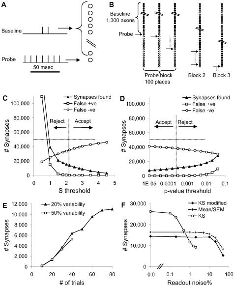
Figure 5. Finding Synapses From the Full Network.

(A) Stimulus design in time. The baseline stimulus had two pulses. The probe stimulus had seven pulses that straddled the baseline. (B) Stimulus design across axons. The baseline stimulus consisted of 1300 axons. The position of the baseline remained the same for 100 different positions of individual probe stimuli. This was referred to as a block of baseline/probe stimuli. Then the baseline was shifted over by 100 positions, and a new block of baseline/probe stimuli was delivered, and so on. (C) Mean/SEM statistic S used to classify synapses. The classification was accepted (vertical dashed line) only if the number of false positives was less than 1% of the number of classified synapses. At high values of S very few synapses were classified at all, and the number of false negatives approached the total number of synapses (horizontal dashed line). (D) Similar classification using the modified Kolmogorov-Smirnov probability p. This statistic correctly classified fewer synapses. (E) Modified KS classification as a function of # of stimulus repeats. The same 1/100 false positive criterion was applied. The results were only slightly affected by variability between neuronal parameters. (F) KS and mean/SEM classification as a function of instrumentation noise (simulated as Gaussian noise with mean zero and the specified standard deviation). The KS statistic did better at low noise, whereas mean/SEM and modified KS methods worked even for high noise levels.