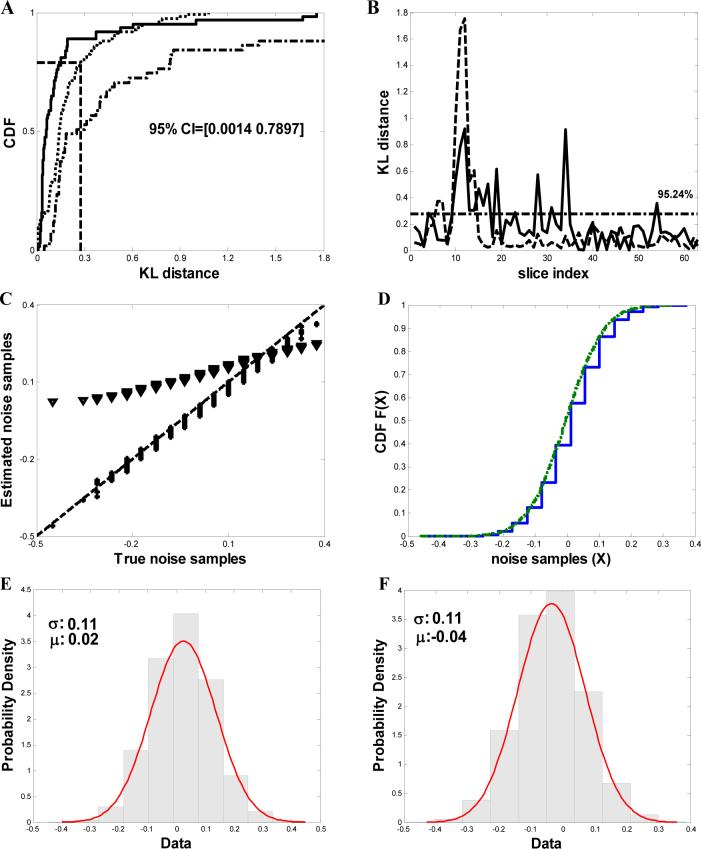
Fig. 2.
Denoising analysis of frozen-hydrated Bdellovibrio cell tomogram from data recorded at liquid nitrogen temperatures (A) Comparison of the cumulative distribution functions (CDF) of the KL-distance D(S̃Ŷi ∥ S̄Ŷi) shown as dotted line (········)(S̃Ŷi and S̄Ŷi are the corresponding probability mass functions of any two randomly chosen partitions S̃Ŷi and S̄Ŷi of the noisy samples SŶi) and D(SŶi ∥ SN̂i shown as solid line  respectively (SŶi and SN̂i are the probability mass functions of SŶi and SN̂i) from the tomogram after denoising with NAD. The 95% confidence intervals are shown. The dashed-dotted line represents the cumulative distribution of the KL-distance using Wiener filtering. (B) Comparison of KL-distances. The solid curve
  represents the KL-distance between random partitions of the raw noise samples and the dotted line (········) represents the KL-distance between true and the estimated noise samples. The horizontal dashed-dotted line depicts the upper confidence values. (C) Quantile-quantile (q-q) plot of true and the estimated noise samples after denoising using NAD denoising algorithm with optimal parameters (*) and using Wiener filtering (▼). The 45° slope line is shown in the plot as a dashed line (----). (D) Comparison of the distributions of true
  and the estimated noise samples (········) after denoising. (E) & (F) Comparison of the probability density functions of true and estimated noise samples. A Gaussian fit is computed with the mean and variance shown in the respective plots.

