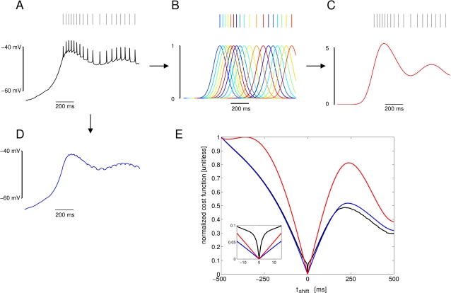
Figure 15. Components of the cost function and how they are calculated.

A) An Example of a membrane potential trace from the LP model with gray bars indicating timing of detected spikes. To obtain the corresponding spike density function (SDF), a Gaussian of fixed width σ = 100 ms and amplitude 1 is added at each time of spike occurrence (B). The colors in (B) illustrate which spike is represented by which Gaussian. The summation of all curves results in the SDF shown in (C). The moving average of the membrane potential is formed by averaging its 100 previous time steps, in this example of about 0.4 ms each (D). E) Illustration of the typical contribution of the cost function components. Here, the time series was time-shifted and compared to an non-shifted version of itself at varying time shifts (x axis; the inset is an enlargement of the region around 0). The dependece of a direct membrane potential cost function on time shift is shown in black (based on the Euclidean distance between all points of the membrane potential and the shifted membrane potential). The dependence of the SDF cost function (the Euclidean distance between all points of the two SDFs) on time shift is shown in red, and the cost for the moving average (the distance between the averaged membrane potentials at varying time shifts) is shown in blue. Note, how both the SDF and moving average widen the “valley” around the minimum where the data is not shifted and thus has 0 distance. It is, therefore, easier to find the minimum with a search algorithm if these types of cost functions are used rather than a direct membrane potential difference. While in this respect similar, the SDF-based distance differs from the distance based on the moving average in that it is sensitive to the existence of spikes. A “naked burst” like shown in Figure 5B for blocked I_Na would, when compared to the control data, lead to small cost for the moving average, but immense cost for the SDF.