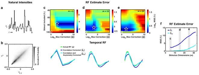
Figure 2. Temporal RF estimates from simulated responses to natural stimuli.

a) 60 sample segment of a time-series of natural intensities taken from the database of van Hateren [16]. b) Two-point distribution of intensities in the natural stimulus. c) Color image showing the (log₁₀) mean squared error between the actual RF used to simulate responses of the LN model to the natural stimulus and RF estimates corrected for stimulus correlations and asymmetries ĝ_cs computed from the simulated responses with different values of θ, defined in terms of the % of stimuli that were included in the RF estimate, and φ, the maximum value for the asymmetry correction. The minimum error is denoted by the star, and the error corresponding to correction for correlations only is denoted by the circle. The actual RF (m = 5) used to simulate the LN model responses to the natural stimulus is shown (green), along with the RF estimated from simulated responses after correction for stimulus correlations only ĝ_c (blue) and correction for stimulus correlations and asymmetries ĝ_cs with optimal values of θ and φ (cyan). d,e) Results for m = 15 and m = 25, presented as in c. f) Mean squared error between actual RFs and RF estimates ĝ_c (blue) and ĝ_cs with optimal values of θ and φ (cyan) for different values of m.