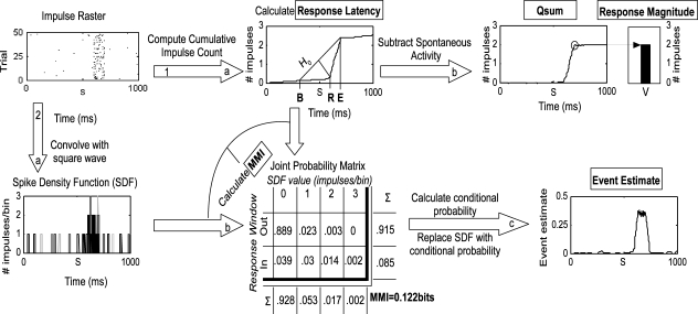
Figure 1.

Methods employed in the analysis. This flow chart illustrates the two principal routes of analysis beginning at the impulse raster. The raster was generated from simulations of Poisson processes with a 0.5 Hz spontaneous rate, 20 Hz stimulus-driven rate, and a 100 ms response duration. The first route has two stages (1a and b) as follows: the raster is converted to a cumulative impulse count by keeping a running tally of the number of impulses over time and averaging across trials. The three-step geometric method is then used to first estimate the response offset (E), bracket the response onset with [B = S − (E − S)], and then find the maximum divergence of the C(T) from the null hypothesis line (H₀) that connects C(B) and C(E). The time of the maximum divergence is R, the response onset. The estimate of the response offset (E) is then improved using a similar technique (not shown, see text for more details). The cumulative impulse count is then converted to the qsum by subtracting time multiplied by the spontaneous rate. The value of the qsum at E is the mean total impulse count. The second route has three stages (2a–c) as follows: the impulse raster is converted to an SDF by convolving it with a fixed-width square-wave function on a trial-by-trial basis (different shades indicate different trials in the plot). The response onset and offset are used to divide the SDF into two ranges according to whether activity is occurring inside or outside the response window. The SDF is sampled every millisecond on every trial to populate a joint probability matrix relating observed values of the SDF (e.g., 1 impulse/bin) to the response window. The marginal distribution for each dimension is calculated by summing across each column and each row. The two marginal distributions are then multiplied to form the expected matrix given random association between SDF values and the response window (not shown). The joint probability matrix and random matrix are used together in calculating MMI as described in the text. The joint probability matrix is converted to a conditional probability by dividing each row by the marginal distribution of SDF values. The values in the bottom row of the resulting matrix replace the matching values in the SDF, thus indicating the probability at each moment in time on each trial that the observed response pattern belongs in the response window. The result is averaged across trials and corrected for spontaneous activity, resulting in the event estimate. In this example, the event estimate reaches and maintains a plateau during the response, as expected given the constant stimulus-driven firing rate in the simulation.