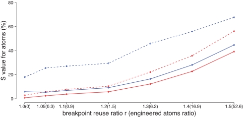
Fig. 7.
Comparison between the infinite-sites algorithm (solid lines) and DUPCAR (dotted lines). Blue lines represent reconstruction of the genome of the Boreoeutherian common ancestor, for which no outgroup is available in this dataset, and the red lines represent the Euarchontoglires ancestor (i.e., the primate–rodent common ancestor). Each data point is the average of 100 simulations, each using ≈2,000 atoms. On the vertical axis, we plot the percentage of atom instances where the true and predicted ancestral genomes disagree, defined as Satom = ((∣R ∪ P∣ − ∣R ∩ P∣)/(∣R ∪ P∣)) × 100%, where R is the set of atom instances in the true ancestral genome, P is the set of atom instances in the predicted genome, and ∣X∣ denotes the size of the set X. The horizontal axis represents variation in the breakpoint-reuse ratio r (35), defined here as r = (2x + 3y)/(a + m − n) where x is the number of two-breakpoint operations in the whole evolutionary history, y is the number of three-breakpoint operations, a is the total number of atoms, m is the number of uses of contig ends as breakpoints, and n is the number of contigs in the root genome. The justification of this formula is that in the infinite-sites model, if we start with n contigs (counted as initial atoms) and an arbitrary number of circular chromosomes (not counted as atoms) in the root genome, then each two-breakpoint operation adds 2 to the quantity a + m, because each breakpoint it uses that is not a contig end adds another atom. Similarly, each three-breakpoint operation adds 3 to the quantity a + m. Finally, when all of the circular chromosomes are hit by rearrangements at least once, we have a total number of atoms a = 2x + 3y + n − m, and hence the breakpoint-reuse ratio (2x + 3y)/(a + m − n) = 1. Any ratio higher than this represents breakpoint reuse. The number in the parentheses is ((no. of engineered atoms used)/(no. of atoms)) × 103 (see Section 9 in SI Appendix).

