

Abstract
The CompuCell3D modeling environment provides a convenient platform for biofilm simulations using the Glazier-Graner-Hogeweg (GGH) model, a cell-oriented framework designed to simulate growth and pattern formation due to biological cells’ behaviors. We show how to develop such a simulation, based on the hybrid (continuum-discrete) model of Picioreanu, van Loosdrecht, and Heijnen (PLH), simulate the growth of a single-species bacterial biofilm, and study the roles of cell-cell and cell-field interactions in determining biofilm morphology. In our simulations, which generalize the PLH model by treating cells as spatially extended, deformable bodies, differential adhesion between cells, and their competition for a substrate (nutrient), suffice to produce a fingering instability that generates the finger shapes of biofilms. Our results agree with most features of the PLH model, although our inclusion of cell adhesion, which is difficult to implement using other modeling approaches, results in slightly different patterns. Our simulations thus provide the groundwork for simulations of medically and industrially important multispecies biofilms.
Key words and phrases: Biofilms, Glazier-Graner-Hogeweg model, cellular Potts model, bacterial growth, computational biology, CompuCell3D
1. Introduction
This paper presents the computational methodology to implement a preliminary model of single-species biofilm growth using the Glazier-Graner-Hogeweg (GGH) model [33, 34, 37],1 as implemented in the CompuCell3D [17, 18, 44] modeling environment.2 Our fairly simple model includes an explicit representation of a nutrient field, but does not include explicit extracellular matrix (ECM). We show that even our simple model reproduces existing results, providing a platform for exploring new phenomenology due to explicit cell shape, ECM properties and multispecies interactions.
A biofilm is an aggregation of microorganisms embedded in a protective and adhesive ECM (also called an extracellular polymeric substance or exopolysaccharide (EPS) matrix) [2]. A biofilm is not a multicellular organism but a community of independent individuals. Although biofilms spontaneously form patterns and structure, no evidence suggests that this formation is the result of a genetically controlled developmental program [51, 78]. Gene expression in biofilms closely correlates with gene expression in stationary-phase bacteria in liquid culture with some degree of anaerobic and iron-limited growth. Biofilms often contain many different species and types of microorganisms, e.g., bacteria, archaea, protozoa, algae, and fungi [20]. They may be structurally and genetically heterogeneous, with complex community interactions and with members of each species performing specialized metabolic functions [14].
Biofilms are very common, existing on almost any solid substrate submerged in, or exposed to, water, from river bottoms to the lining of the gut [14]. They can also form floating mats on liquid surfaces. Even single-species biofilms exhibit a wide variety of morphologies, making them interesting examples of spontaneous patterning (pattern formation) [13, 19, 23]. Biofilms have no “typical” structure, since, like trees in forests, biofilms can produce all sorts of shapes. These shapes depend on multiple factors including cell motility, the existence of multiple cell phenotypes, the nature of the secreted ECM, flows in the surrounding liquid medium, the properties of the surface on which the biofilm grows, and mass transport in the liquid medium and ECM. Thus biofilms serve as interesting models of the origin of multicellularity, cooperativity, and ecological specialization, making simulations of multispecies biofilms potentially useful in the study of these basic biological questions.
Biofilms contribute to a host of industrial and medical problems, ranging from ship fouling to antibiotic resistance and tooth decay. Biofilms also present a unique opportunity in environmental technologies for cleanup and containment of hazardous waste. Since biofilms are involved in about 80% of microbial infections in humans [1], a realistic understanding of how biofilms grow3 and how they contribute to antibiotic resistance would be of practical value.
Because of the difficulty of observing and controlling real biofilms, they have attracted much attention from modelers wishing to clarify the roles of different biological and physical mechanisms in determining biofilm properties. Biofilm models generally divide into cell-centered models with discrete cells (cellular automata [8, 39, 69] or individual-based models [25, 52, 85]), and continuum models [3, 26, 28, 84]. Hybrid models combine discrete cells with a continuum representation of the ECM and/or extracellular fluid [4] or with PDEs for reaction-diffusion [66, 67, 68]. The first continuum, one-dimensional (1D) mathematical models of biofilms considered only gradients perpendicular to the biofilm-liquid interface [83]. Later, two-dimensional (2D) models based on physical principles explored the ways lateral gradients create biofilm structures [8, 25, 28, 39, 52, 66, 67, 68, 69]. These models addressed the spontaneous formation of heterogeneous structures, the influence of flow-induced breakage and substrate gradients, and the role of pores in biofilms [82].
However, we still lack both a fundamental theory and accurate experimental observations of biofilm growth [82]. In addition, most existing models have certain limitations that may impair their viability in describing complex real biofilms. Many cell-centered and hybrid models describe individual cells as points [66] or spheres [4]. However, cell shape can be essential in biological development,4 and changes in cell shape reflect the elastic properties of cells.
Thus, this paper takes a cell-oriented, hybrid approach to biofilm modeling [56]. We treat cells as macroscopic objects with mechanical properties.5 Since the size of substrate molecules is small compared to the size of the biofilm cells, we treat substrates as continuous diffusive fields.6 The main goal of this paper is to validate our GGH-based approach by reproducing known simulation results for single-species biofilms. This validation is essential to future studies, which will apply the GGH model to multispecies biofilms, where differences in cell adhesion and elasticity between various types of cells may greatly affect biofilm development. Because the methods against which we are benchmarking do not include explicit cell shape, we model cells as deformable bodies rather than cells with a fixed shape, as in real bacteria. However, we can easily add explicit cell shapes in future simulations. Treating cells as extended, deformable objects allows us to investigate the role in biofilm formation of cell-cell and cell-ECM adhesion, which are crucial in many types of biological pattern formation [76]. Although analyzing the effects of cell adhesion does not require spatially extended objects [12], our approach allows us to introduce elasticity and surface tension directly, in terms of free energies [33]. Furthermore, the GGH model allows us to include in a simple and physically correct fashion many other biologically relevant phenomena, e.g., cell polarity and compartmental cell structure [6].
2. The PLH biofilm model
Overall, our choice of biological mechanisms follows the very successful model of Picioreanu, van Loosdrecht, and Heijnen (PLH) [66, 67], with the important difference that our cells are extended, elastic, adhesive objects. We do not model ECM explicitly. However, we include it implicitly in the form of a cell-medium adhesion coefficient in the GGH effective energy (see section 3). Thus, our GGH biofilm cells correspond to clusters of real biofilm cells surrounded by a thin layer of ECM.
The hybrid differential-discrete PLH model [66, 67] focuses on the development of single-species biofilms containing Nitrosomonas europaea or Nitrobacter agilis, using kinetics derived from [7, 24]. A 2D rectangular mesh discretizes space. Two variables represent the state of the simulated biofilm: the soluble substrate7 concentration S, and the biomass density C. In addition, the solid component matrix c stores information about the occupation of space. The quantities S and C vary between 0 and 1, while the occupation state c takes either the value 0 (an unoccupied site) or 1 (a site with biomass). The variables S and C are defined as
| (1) |
| (2) |
where cX is the biofilm density, cXm is the maximum biomass density in a colony, cS is the local substrate concentration and cS0 is the substrate concentration in the bulk liquid. The substrate concentration cS in 2D obeys the diffusion equation
| (3) |
where DS is the substrate diffusion coefficient, and the substrate consumption rate, rS, depends on both cS and the biomass density in the biofilm, cX. By construction, the PLH model does not include the effective surface energy between cells or between cells and the bulk liquid.
In the absence of detailed experimental data, most biological models, including the PLH model, assume a Monod-like saturation function to describe the substrate consumption rate [67]:
| (4) |
where μm denotes the maximum specific growth rate, YXS is the growth yield (amount of biomass produced per unit of substrate), mS is the maintenance coefficient and KS is the Monod saturation constant [67]. The equation for biomass balance is
| (5) |
where the net rate of biomass formation, rX, is
| (6) |
Combining equations (4)–(6) gives
| (7) |
which is the same as
| (8) |
At low substrate concentrations, this model allows negative biomass growth (shrinkage), while at high substrate concentrations the biofilm growth rate reaches an observable maximal value. To simulate cell division and mechanical elasticity, when the biomass concentration C reaches its maximum value 1 at a given location, it divides into two equal parts. The first stays where it started, while the other moves to a randomly chosen, adjacent grid element, updating the occupation matrix c through a cellular-automaton mechanism [67]. Specific boundary conditions govern substrate uptake from the environment. For a biofilm forming on a solid support, the substrate concentration is constant and maximal (S = 1) outside the aqueous medium [66].
In the PLH model, biofilm morphology depends on a single parameter, the nondimensional ratio of the maximum biomass growth rate to the maximum substrate transport rate. In terms of the quantities introduced in the preceding paragraphs, this ratio (called the Growth Group Parameter) is [66]
| (9) |
where lz is the maximum biofilm thickness. If G is small, the substrate diffuses fast enough that an appreciable quantity reaches all regions of the growing biofilm, and its isoconcentration lines are flat and horizontal. Therefore, the growing biofilm remains essentially compact and flat. For larger values of G, faster substrate consumption prevents the substrate from reaching all regions of the growing biofilm, inducing competition for the substrate. In this case, both the substrate distribution and the biofilm density become more irregular, and deep vertical channels (valleys) form in the biofilm density in a fingering instability [21, 38, 60, 64]. When G is very large, growth is very slow and filamentous structures form. This general behavior holds in both 2D and 3D simulations [66].
3. The GGH biofilm model
A general model of a growing biofilm needs three main elements [26]. First, a transport mechanism like diffusion or advection-diffusion must bring growth substrates (e.g., oxygen, nutrients) to the cells in the biofilm. Second, cells must grow and proliferate while consuming growth substrates. The third and least understood element is biofilm loss due to breakage or cell death. In addition to these fundamental mechanisms, we could explore the effects of other factors such as cell-cell or cell-ECM adhesion,8 or the elastic reactions of biofilms to fluid-flow-generated shear stress.
Our mathematical model of biofilm growth adapts the PLH hybrid model to the Glazier-Graner-Hogeweg (GGH) model, also known as the cellular Potts model (CPM), which includes subcellular, cellular, and continuum mechanisms such as cell adhesion, growth and division, diffusion of chemicals, chemotaxis (movement of cells up or down a gradient of an extracellular diffusing chemical), and haptotaxis (movement of cells due to changes in cell-cell and cell-ECM adhesion, ECM stiffness, or ECM-bound chemicals). GGH applications include models of Hydra vulgaris regeneration, cell motility [62], cell deformation [72], chick embryo mes-enchymal chondrogenesis [17, 44], growth [71] and cell motility [63], tumor growth [47, 77], embryonic convergent extension [86], vasculogenesis [57], avascular tumor growth [27], cancer invasion [79, 80], aggregation, slug behavior and culmination in Dictyostelium discoideum [46, 53, 54, 55, 74], the liquid-like behavior of chick-cell aggregates [10], chick limb growth [71], engineering biological structures using self-assembly [45, 65], directional sorting of chemotactic cells [49], evolutionary mechanisms [40, 41, 42], foams [48, 73], and viscous flow [22]. Figure 1 shows a few biological applications of the GGH.
Figure 1.
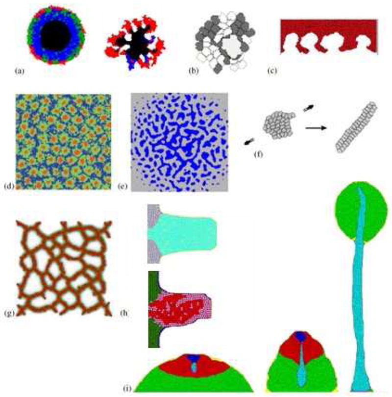
GGH modeling in developmental biology: (a) model of stable and branching avascular tumors (based on the model of [5]); (b) clonal selection of B-cells in a germinal center through competition for contact with a large antigen-presenting cell [50]; (c) tumor invasion [81]; (d) Delta-Notch-mediated stem-cell cluster-size control in the human interfollicular epidermis [75]; (e) mesenchymal condensation due to cell-ECM interactions [88]; (f) convergent extension in embryonic development [87]; (g) endothelial cells, secreting an analog of VEGF-A, chemotactically aggregate to form a vascular network [58]; (h) chick limb growth [71] and chondrogenic condensation; (i) formation of a fruiting body in Dictyostelium discoideum [54].
GGH models include objects, interaction descriptions, dynamics and initial conditions. Objects in a GGH model can be generalized cells or fields. Generalized cells are spatially extended domains, which reside on a single cell lattice and may correspond to clusters of biological cells, biological cells, subcompartments of biological cells, or to portions of noncellular materials, e.g., ECM, fluids, solids, etc. [6, 33]. Generalized cells can carry within them chemical concentrations, state-descriptors (e.g., time since last mitosis), descriptions of biochemical interaction networks, etc.
Fields are continuously variable concentrations, each of which resides on its own lattice. Fields typically represent chemical diffusants, nondiffusing ECM, etc. Multiple fields can be combined to represent materials with textures, e.g., fibers.
Interaction descriptions and dynamics define how the various objects behave both biologically and physically. For generalized cells, these behaviors and interactions are embodied primarily in the effective energy (also known as the CPM Hamiltonian), which determines a generalized cell’s shape, motility, adhesion and response to extracellular signals [33]. Local minimization of the effective energy [76] drives most pattern dynamics [33, 34, 37]. The effective energy mixes true energies, such as cell-cell adhesion, and terms that mimic energies, e.g., the response of a cell to a chemotactic gradient of a field. Mathematically, N spatially extended cells indexed by σ lie on a 2D or 3D lattice; the value at a lattice site (pixel) i⃗ is σ if this site lies in cell σ. A collection of connected lattice sites with the same index represents a cell, as shown in Figure 2. To each cell we associate a cell type τ. Different cells can have the same value of τ.
Figure 2.
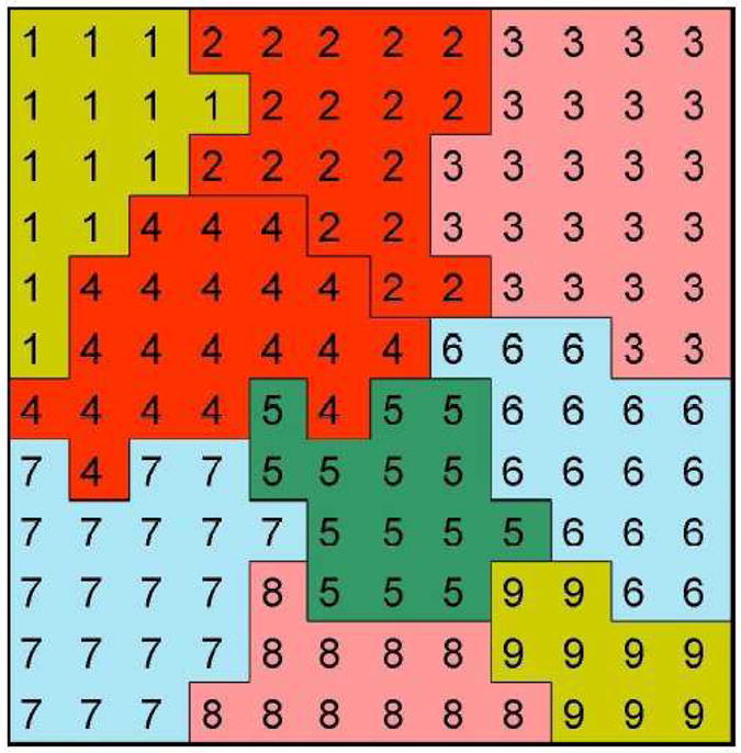
A typical GGH configuration in 2D showing portions of nine generalized cells. The numerals indicate index values. The colors indicate cell types. A generalized cell is a collection of connected lattice sites (squares) with the same index value. The number of lattice sites in a cell is its volume and the number of lattice links on its boundary (interfaces with other indices) is its surface area.
A typical effective energy in our simulations includes two main terms [33, 34, 37]:
| (10) |
The first term describes the surface energy between cells, and between cells and their environment, in terms of symmetric surface energies J(τ, τ′) = J(τ′, τ) [33, 34, 37]. To calculate the energy resulting from cell-cell adhesion we consider first-, second-, and third-nearest neighbor lattice sites, which reduces lattice anisotropy effects compared to first-neighbor calculations [43].9 The second term corresponds to the compressibility of the cells and prevents cell disappearance; V(σ) is the volume in lattice sites of cell σ, Vt its target volume, and λV (τ) the strength of the volume constraint.10
Instead of the surface-adhesion coefficients J(τ, τ′), we can use surface tensions γ(τ, τ′), defined as
| (11) |
Negative surface tensions correspond to mixing or dispersing cells, while positive surface tensions correspond to cell sorting.
We simulate growth of cells by increasing their Vt by a function f which typically depends on the local concentrations of chemicals C that induce growth and the internal state of the cell [71]:
| (12) |
If a cell reaches a given doubling volume, it divides and splits along a random axis (with no splitting orientation) into two cells with equal target volumes of one half the parent-cell volume (we can easily add oriented cell division, but it is not included in the PLH model [66, 67]). Adding constraints to the effective energy can describe many other cell properties, including osmotic pressure and membrane area [17, 44], the average shape of the cells [57, 86], chemotaxis [40, 54], viscosity and advective diffusion [22], rigid-body motion [6], and cell compartments for the simulation of polarized cells, e.g., in epithelia [11].
The cell lattice evolves through attempts by generalized cells to extend their boundaries into neighboring lattice sites, slightly displacing the generalized cells which currently occupy those sites. These extensions change the effective energy, and we accept each one with a probability that depends on the resulting change of the effective energy according to an acceptance function [33]. Thus, the cell lattice evolves to minimize the total effective energy [32, 36] (we can translate the effective energy rigorously into a force-based formalism if we choose, but the effective-energy formalism is more convenient). The rearrangement dynamics uses a relaxational Monte-Carlo-Boltzmann-Metropolis dynamics [33, 34, 37, 59], modified so that averaged local movements of cell boundaries obey the overdamped force-velocity relationship (modified Metropolis dynamics):
| (13) |
where μlocal is the local mobility of the object experiencing the force and υ⃗ the local boundary velocity. The cells rearrange their positions to minimize the total effective energy [76]. At each step we randomly select a lattice site i⃗ and attempt to change its index from σ(i⃗) to the index σ′= σ(i⃗′) of an arbitrary lattice site i⃗′ in its third-order neighborhood (a lattice site which connects to i⃗ by a side, edge, or corner). We accept the change with a probability P:11
| (14) |
where Δℋ is the difference in effective energy produced by the change, θ is the Heaviside step function, and T is a parameter corresponding to the amplitude of cell fluctuations [61].12 One Monte Carlo Step (MCS) by default corresponds to n index-change attempts, where n is the total number of lattice sites (however, in our biofilm simulations, we will define a Monte Carlo Step as index-change attempts; see section 4).
Auxiliary equations describe cells’ absorption and secretion of diffusants and extracellular materials (i.e. their interactions with fields), state changes within the cell, mitosis, and cell death [33]. Usually, state changes affect generalized-cell behaviors by changing the parameters present in the effective energy (e.g., the surface density of a particular cell adhesion molecule). Fields evolve due to cells’ secretion and absorption at their boundaries, and diffusion, reaction and decay under the control of PDEs. The initial condition specifies the initial configurations of all generalized cells and fields, all internal states related to auxiliary equations and any other information required to completely describe a model.
If, as in the PLH papers cited, simulated bacteria are aerobes and we assume that they have plenty of nutrients so their growth is limited only by their oxygen supply, our substrate field (O) represents oxygen. We could also use it to represent a key nutrient to model anaerobic bacteria growing in a nutrient-limited environment. Our single-species biofilm model includes four types of generalized cell, representing: biofilm cells (b), a substrate source (o), a solid bottom (s), and an aqueous medium (m) submerging the growing biofilm.13 The substrate-source and solid-bottom cells are frozen, i.e. they do not exchange pixels with other cells. Fields do not have an excluded volume, i.e. they can co-occupy space with cells. We treat the medium as a large generalized cell without a volume constraint. We can regard the medium as all space in the cell lattice that is not occupied by other generalized cells. Treating the medium as a generalized cell allows us to represent the surface tension of real cells. Figure 3 shows the initial 2D configuration for our simulations.14 The dimension of the domain in pixels is 200 × 100 × 1 (the z-axis is perpendicular to the page). We are free to assign the length scale and time scale in the simulation, which fixes the other parameters. We set 1 pixel to 4μm, so the vertical height of the simulation domain is 400μm, as in [66], and 1 MCS to 3000s, so 1000 MCS corresponds to approximately 35 days. Each biofilm cell initially occupies a 2 × 2 × 1 cube, which is approximately 10 times larger than the real bacterial cells.15 The initial value of Vt for biofilm cells is equal to their initial volume. We simulate growth of biofilm cells by applying equation (8) in the equivalent form:
| (15) |
Figure 3.
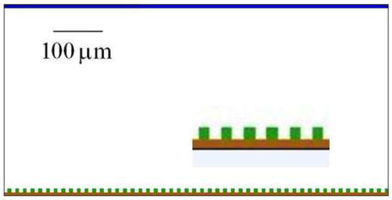
The initial lattice configuration, with biofilm cells (colonists) at the bottom, sitting on a flat solid, and generalized cells producing substrate at the top. The space between the cells is aqueous medium with an initially homogeneous concentration of substrate. The vertical height corresponds to 400μm and the horizontal length to 800μm. The inset inside the simulation domain shows an enlarged fragment of the solid bottom and a few biofilm cells.
In the hybrid PLH model [66, 67], cells divide when the local value of C reaches 1. In the GGH model, biofilm cells divide when V reaches the doubling volume Vd, which is twice their initial Vt. Therefore, both C and Vt represent the closeness of cells to division, which justifies equation (15). We can rewrite equation (15) in a form which explicitly depends on G:
| (16) |
where
| (17) |
Equations (3) and (4) give
| (18) |
Since cX and Vt represent the same object, they are proportional to each other:
| (19) |
We rewrite equation (18):
| (20) |
where the effective decay constant k is
| (21) |
which shows k’s dependence on G. In our simulations, we simplify equation (21) by setting Vt = 3Vd/4, which corresponds to the average cell volume. We also ignore cell loss by setting mS = 0,16 and do not model cell death. Equation (21) has two limiting cases: . In the first case, k does not depend on S, so the second term in the right-hand side of equation (20) is proportional to S, which represents substrate decay. In the second case, the decay constant k is proportional to , so the second term in the right-hand side of equation (20) is independent of S, which represents substrate consumption. We effectively combine both limiting cases by rewriting equation (20) as
| (22) |
where
| (23) |
and
| (24) |
The substrate-source cells, representing the contact of the liquid medium with oxygen in the air, secrete substrate, which diffuses into the medium and biofilm cells. Secretion occurs at a constant rate, and we keep the substrate concentration S everywhere below a threshold value 1 (corresponding to the maximum solubility of substrate in water) by checking whether S > 1 anywhere. If so, we set S = 1 at those points. A constant secretion rate for substrate would implement a constant-flux boundary. However, the requirement S ≤ 1 yields a constant-concentration boundary, in agreement with a constant oxygen partial pressure in the surroundings. This algorithm means that the net supply of substrate increases as its consumption by biofilm cells increases and also increases as the separation between the biofilm and the liquid surface decreases, which is realistic for biofilms growing in thin liquid films, where the substrate concentration at the surface is always saturated. It does not describe well a biofilm growing deep under water, where the maximum substrate concentration is well below saturation. The substrate distribution is initially homogeneous and saturated, so S = 1 everywhere. Substrate-secreting generalized cells increase the concentration of substrate at a fixed rate in the pixel corresponding to their center of mass. Biofilm cells consume substrate by secreting negative amounts of substrate at their centers of mass.17 Substrate diffuses on the field lattice using a forward-Euler algorithm run N′ times per MCS, where N′ depends on the time and distance scales we have chosen, and the substrate diffusion constant, DS. We use no-flux boundary conditions at the bottom of the simulation domain, and periodic boundary conditions at the sides to simulate a large biofilm.
We must specify all parameters in our simulations in GGH units: pixels, MCS,.... In the absence of experimental measurements of these parameters, we choose them in a range which exhibits the general classes of behaviors observed experimentally. The fluctuation amplitude T rescales the surface-adhesion coefficients J(τ, τ′) and the volume-constraint coefficient λV. Here, we choose these values to prevent cells from disappearing or freezing, and use the hierarchy of surface-adhesion coefficients to keep the cells from desorting (i.e. to keep the bacterial cells from floating off into the liquid medium). Thus, for each pair of generalized-cell types τ and τ′ we set J(τ, τ) ≤ J(τ, τ′) and J(τ′, τ′) ≤ J(τ, τ′). For the biofilm cells we also have , where is on the order of the approximate critical surface tension below which cell dissociation occurs (the factor of 12 is the number of neighbors in the 2D third-order neighborhood), which keeps them from dispersing into the medium [34]. In the GGH model, stronger adhesion corresponds to lower values of the surface energy J. Since bacterial cells are viscoelastic, we could, in principle, obtain their surface adhesion coefficients from parallel-plate compression experiments [10, 29, 30, 31].
Unless we specify otherwise, we use the following values for the cell-cell and cell-medium adhesion coefficients, which satisfy the above inequalities [35]:
| (25) |
The other J(τ, τ′) are irrelevant, so we set them to zero. We also set T = 10 following [34, 37]. Our choice of parameters is somewhat arbitrary, since only experiments can provide their exact relative values. We choose λV = 40, which prevents the cells from disappearing and makes them fairly rigid. We take the parameters in equations (1)–(8) from [66], except for mS, which we set to 0.18 We control the value of the non-dimensional parameter G in equation (9) by changing cS0.
4. Implementing the GGH mathematical model in CompuCell3D
Now that we have defined our mathematical model of biofilm growth, we must translate it into a simulation. Our simulations use CompuCell3D [15, 16, 17, 18, 44], an open-source, multimodel software framework for simulation of the development of multicellular organisms.19 The great advantage of the CompuCell3D implementation of the GGH is that it uses simple CompuCell3D markup language (CC3DML) to specify models, allowing easy model sharing and validation [6]. CC3DML is simple to read and write and fairly compact.
To illustrate the translation of our model into CC3DML code, we review the derivation and meaning of the most relevant parts of the model. We provide the complete CC3DML code corresponding to our simulation with G = 10 in Appendix A; all the CC3DML code, the plugins and steppables, and the PIF and TXT files used in our simulations are available for download from http://www.compucell3d.org/Models/biofilm.
The first section of a CC3DML configuration file defines the global parameters of the lattice and the simulation:
〈CompuCell3D〉
〈Potts〉
〈Dimensions x=“200” y=“100” z=“1”/〉
〈Steps〉20000〈/Steps〉
〈Temperature〉10〈/Temperature〉
〈Flip2DimRatio〉0.01〈/Flip2DimRatio〉
〈Boundary_x〉Periodic〈/Boundary_x〉
〈Boundary_y〉NoFlux〈/Boundary_y〉
〈Boundary_z〉NoFlux〈/Boundary_z〉
〈FlipNeighborMaxDistance〉2.1〈/FlipNeighborMaxDistance〉
〈/Potts〉.
The line 〈Dimensions x=“200” y=“100” z=“1”/〉 declares the dimensions of the lattice to be 200 × 100 × 1, i.e. the lattice is 2D and extends in the xy plane. The basis of the lattice is 0 in each direction, so the lattice sites in the x and y directions have indices ranging from 0 to 199 and from 0 to 99, respectively.
The lines 〈Steps〉20000〈/Steps〉 and 〈Temperature〉10〈/Temperature〉 tell Compu-Cell3D that the simulation should last 20000 MCS, with the fluctuation amplitude in equation (14), T = 10. The line 〈Flip2DimRatio〉0.01〈/Flip2DimRatio〉 tells Com-puCell3D that it should make 0.01 times the number of lattice sites (199 × 99 × 1) index-change attempts per MCS. The purpose of this definition is to model processes with fast time scales, in our case allowing for flexible definition of the diffusion constant of the substrate. In our case, the diffusion constant of the substrate is 100 times larger than the nominal value in the code (see below). The next line 〈FlipNeighborMaxDistance〉2.1〈/FlipNeighborMaxDistance〉 specifies the range of interactions (in pixels) to be third neighbor. A value of 1 corresponds to nearest-neighbor interactions. The longer the interaction range, the more isotropic the simulation and the slower it runs. If the interaction range is comparable to the cell size, apparently nonadjacent cells may contact each other. The CC3DML tags 〈Boundary_x〉, 〈Boundary_y〉 and 〈Boundary_z〉 impose boundary conditions on the lattice. In our case, the x axis is periodic; so, for example, pixel (0, 1, 1) neighbors pixel (199, 1, 1), while the y and z axis boundaries have no-flux boundary conditions.
The second section of the CC3DML file contains plugins, which CompuCell3D refers to every time it calculates the effective energy in equation (10). The plugins vary from simulation to simulation and define many of the types, behaviors and interactions of objects used in a given simulation. The ability to specify dynamically plugins (and steppables, see below) gives CompuCell3D its flexibility.
The CellType plugin informs CompuCell3D what generalized-cell types we are using in the simulation:
〈Plugin Name=“CellType”〉
〈CellType TypeName=“Medium” TypeId=“0”/〉
〈CellType TypeName=“Oxygen” TypeId=“1” Freeze=“”/〉
〈CellType TypeName=“Biofilm” TypeId=“2”/〉
〈CellType TypeName=“Support” TypeId=“3” Freeze=“”/〉
〈/Plugin〉.
Each line contains the name of a type that the simulation uses and assigns it to an integer-valued TypeIdpeId. Medium is traditionally assigned a TypeIdpeId = 0 (this type index does not have a volume constraint by construction). In our simulations we create four cell types, Medium, Oxygen, Biofilm, and Support. Oxygen cells represent air above the liquid Medium in which Biofilm cells grow. Like Support cells, they are frozen; that is, they do not move by exchanging pixels with other generalized cells.
The Contact plugin defines the boundary energies J(τ, τ′) between cells of different types and the interaction range (Depth) of the neighborhood used in the contact-energy summation in equation (10):
〈Plugin Name=“Contact”〉
〈Energy Type1=“Biofilm” Type2=“Medium”〉16〈/Energy〉
〈Energy Type1=“Biofilm” Type2=“Biofilm”〉8〈/Energy〉
〈Energy Type1=“Biofilm” Type2=“Support”〉4〈/Energy〉
…
〈Depth〉2.1〈/Depth〉
〈/Plugin〉.
The VolumeLocal plugin defines the volume-constraint term in equation (10):
〈Plugin Name=“VolumeLocal”〉
〈LambdaVolume〉40〈/LambdaVolume〉
〈/Plugin〉.
The CenterOfMass plugin enables CompuCell3D to track the center of mass of each cell, for example, to control cell growth (see below):
〈Plugin Name=“CenterOfMass”/〉.
The Mitosis plugin defines the doubling volume at which a Biofilm cell divides into two cells with equal volumes:
〈Plugin Name=“Mitosis”〉
〈DoublingVolume〉8〈/DoublingVolume〉
〈/Plugin〉.
The NeighborTracker plugin enables CompuCell3D to track all neighbors of each cell:
〈Plugin Name=“NeighborTracker”/〉.
The third section of the CC3DML file contains steppables. The PIFInitializer steppable, executed only once at the beginning of a simulation, defines the initial conditions of the cell lattice:
〈Steppable Type=“PIFInitializer”〉
〈PIFName〉Biofilm.PIF〈/PIFName〉
〈/Steppable〉.
A PIF file sets the initial cell lattice configuration for the simulations, and for n generalized cells contains at least n lines, each of which consists of: the index of a generalized cell, the cell type, and the range (in pixels) this cell occupies on the lattice (xmin, xmax, ymin, ymax, zmin, zmax). Using multiple lines/cell allows specification of arbitrary geometries. In our simulations we begin with 50 bacterial clumps distributed uniformly along the bottom (see Figure 3).
CompuCell3D executes the remaining steppables once at the conclusion of every MCS. The FlexibleDiffusionSolverFE steppable introduces fields of chemicals and defines their secretion, consumption, diffusion and decay, in this case, implementing equation (18):
〈Steppable Type=“FlexibleDiffusionSolverFE”〉
〈DiffusionField〉
〈DiffusionData〉
〈FieldName〉Oxygen〈/FieldName〉
〈DiffusionConstant〉0.15〈/DiffusionConstant〉
〈DecayConstant〉0.0015〈/DecayConstant〉
〈ConcentrationFileName〉Oxygen.TXT〈/ConcentrationFileName〉
〈/DiffusionData〉
〈SecretionData〉
〈Secretion Type=“Oxygen”〉1〈/Secretion〉
〈Secretion Type=“Biofilm”〉−0.0006〈/Secretion〉
〈/SecretionData〉
〈/DiffusionField〉
〈/Steppable〉.
The DecayConstant corresponds to k1 in equation (22) and the SecretionData constant for Biofilm cells to k2. The Oxygen.TXT file sets the initial distribution C(x, y, z) of the substrate, with the format: x, y, z, C(x, y, z). In our simulations the initial field is 1 everywhere, representing oxygen saturation in the medium.
Finally, the TargetVolume steppable defines the growth of the Biofilm cells in response to substrate:
〈Steppable Type=“TargetVolume”〉
〈InitialTargetVolume Type=“Biofilm”〉4〈/InitialTargetVolume〉
〈Growth Type=“Biofilm” Field=“Oxygen” GrowthRate=“1” Saturation=“0.033”/〉
〈/Steppable〉.
In this sample program, the Biofilm cells grow under the influence of Oxygen, according to equation (16), where GrowthRate corresponds to μm and Saturation to . The CC3DML file ends with the line:
〈/CompuCell3D〉.
5. Results
In this section, we explore how the morphology of the growing simulated biofilm depends on model parameters, in particular, the dimensionless parameter G in equation (9), which Picioreanu, van Loosdrecht, and Heijnen identified as controlling the selection of flat-interface vs. fingered growth in their hybrid model [66, 67]. Figure 4 shows the terminology we use in this paper to describe the morphology of simulated biofilms and the color code for substrate concentration in Figures 5–16. The leading edge is the vertical position of the highest point in the biofilm. The trailing edge is the average position of the narrowest part of the fingers, or, if fingers are convex, the lowest point occupied by medium. The small white square shows the generalized-cell size. In the following figures, we represent areas containing biofilm cells with white hatch lines, and the biofilm-medium interface as a white boundary line. We do not show the boundaries of individual biofilm cells because they are too small on the scale of the figure. We also show the spatial distribution of the substrate: red–high concentrations (S ~ 1), blue–low concentrations (S ~ 0.1), black–almost no substrate (S ~ 0).
Figure 4.

(a) Terminology describing the morphology of simulated biofilms. (b) Color code for substrate concentrations in Figures 5–16.
Figure 5.

Flat-interface biofilm (white hatch lines) growth in a 2D biofilm simulation with G = 1, J(b, m) = 16 and Rcp = 0.6 (see equation (28)). See equation (25) and text for other parameter values. The morphology is almost flat (growth-limited regime). Colors represent substrate concentration; see Figure 4(b).
Figure 16.

Concave rough-finger biofilm (white hatch lines) growth in a 2D biofilm simulation with G = 50, J(b, m) = 8 and Rcp = 0.39 (see equation (28)). See equation (25) and text for other parameter values. The weaker cell-medium surface tension results in more, narrower, fingers, with relatively narrower valleys, than in the corresponding high-surface-tension G = 50 simulation in Figure 11. Note the greater irregularity of the finger shapes and their rougher surfaces. Colors represent substrate concentration; see Figure 4(b).
For G < 10, the biomass growth rate limits the growth dynamics (growth-limited regime). The substrate penetrates most of the biofilm and reaches most cells. In this case, the simulated biofilms are dense, compact and fast-growing. Growth continues even at the bottom of the valleys between protrusions, resulting in ripples rather than fingers. For G = 1, diffusion is so strong that no valleys form and the biofilm-medium interface remains flat. The isoconcentration lines of the substrate remain essentially horizontal. For G = 2 and G = 5, the biofilm-medium interface becomes rippled. The isoconcentration lines of the substrate curve slightly, following the biofilm-medium boundary. Figures 5, 6, and 7 show simulations with G = 1, 2, and 5, respectively.
Figure 6.

Rippled biofilm (white hatch lines) growth in a 2D biofilm simulation with G = 2, J(b, m) = 16 and Rcp = 0.76 (see equation (28)). See equation (25) and text for other parameter values. The ripples are smooth (growth-limited regime). Colors represent substrate concentration; see Figure 4(b).
Figure 7.

Rippled biofilm (white hatch lines) growth in a 2D biofilm simulation with G = 5, J(b, m) = 16 and Rcp = 0.95 (see equation (28)). See equation (25) and text for other parameter values. The ripples turn into wide convex fingers (growth-limited regime). Colors represent substrate concentration; see Figure 4(b).
Figure 8 shows the time evolution of a simulated biofilm for G = 10. For this value of G, the substrate penetrates several cell diameters into the surface layer of the biofilm. The case G = 10, as we will see below, is a border between two different morphological regimes. As in Figure 9, adapted from [66], the biofilm’s structural complexity increases continuously in time. Initially, the substrate penetrates throughout the biofilm colonies, which grow in all directions. As they grow, the cells consume substrate and the substrate concentration develops a gradient, increasing in the vertical direction. As the biofilm thickens, cells in regions which thicken faster due to statistical fluctuations (protrusions) experience higher concentrations of substrate than others. These cells produce new biomass more quickly, while the cells in the valleys (horizontal locations where the interface between biofilm and medium lags significantly behind the highest local vertical position of the biofilm, as in viscous fingering [21, 38, 60, 64]) experience an environment depleted in substrate, begin to starve, and grow slowly or cease to grow, so the space between growing biofilm clusters fills slowly or not at all with new cells. The valleys deepen and the biofilm becomes more irregular. The isoconcentration lines of the substrate are more curved than for G = 5. This fingering instability generates the fingers observed in experimental biofilms.
Figure 8.

Convex-finger biofilm (white hatch lines) growth in a 2D biofilm simulation with G = 10, J(b, m) = 16 and Rcp = 1.06 (see equation (28)). See equation (25) and text for other parameter values. The fingers are usually convex and the valleys do not pinch off. Colors represent substrate concentration; see Figure 4(b).
Figure 9.
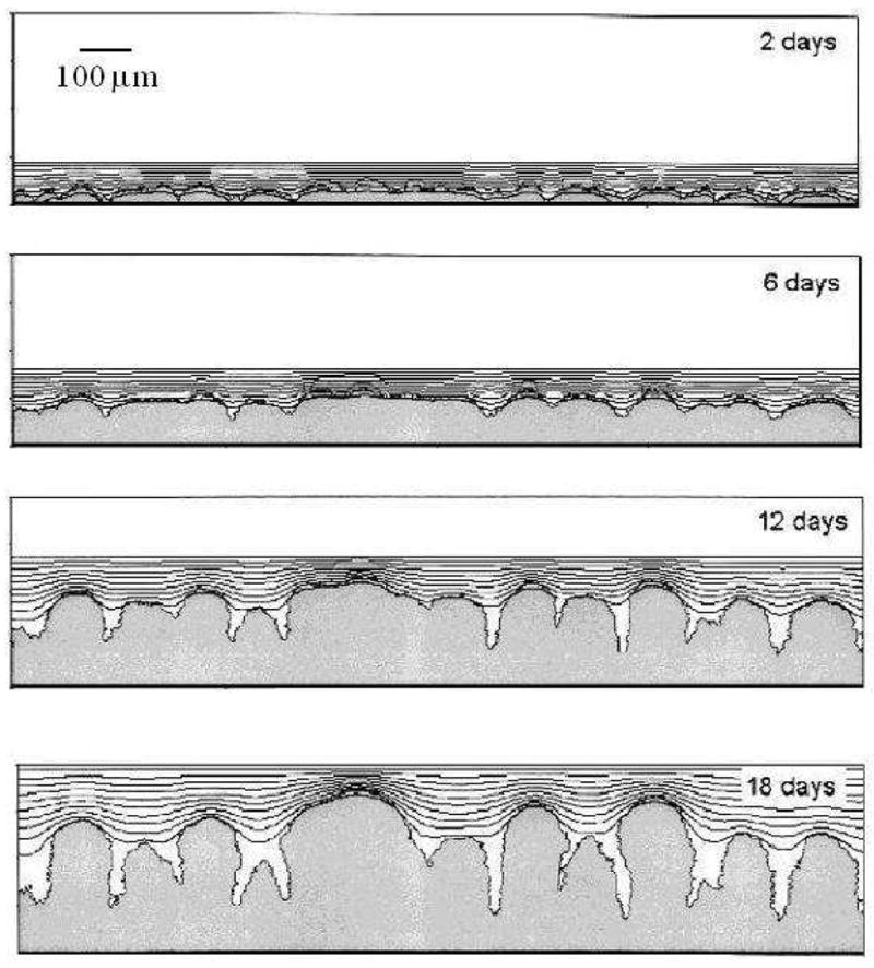
Finger-biofilm growth in the 2D PLH model with G = 10. Isolines represent the substrate concentration. Adapted from [66].
For G > 10, we find a substrate-transport-limited regime: the substrate transfer rate, not the biomass growth rate, limits the growth dynamics. The substrate penetrates thin layers of biofilm, but less substrate reaches deeper layers. Therefore, the valleys between biofilm protrusions are wider and deeper and the structure of the biofilm is more finger-like than for G = 10. Cells in the valleys cease to grow and the fingers develop concave necks. The biofilm fingers grow more slowly than for smaller values of G (reaching the top of the simulation domain after a larger number of MCS). The bigger G, the narrower the fingers and the greater the space between them. The neck of the finger also becomes narrower with respect to the width of the finger. Figures 10 and 11 show simulations for G = 20 and G = 50, respectively. At G = 50, the substrate consumption rate relative to biofilm growth is so large that more cells starve (they do not die in our model, but they do stop dividing) and the simulated biofilm produces fewer fingers. As a result, the isoconcentration lines of the substrate curve significantly, because high concentrations of substrate penetrate into the larger valleys.
Figure 10.

Concave-finger biofilm (white hatch lines) growth in a 2D biofilm simulation with G = 20, J(b, m) = 16 and Rcp = 1.12 (see equation (28)). See equation (25) and text for other parameter values. The fingers are concave (substrate-transport-limited regime). Colors represent substrate concentration; see Figure 4(b).
Figure 11.

Concave-finger biofilm (white hatch lines) growth in a 2D biofilm simulation with G = 50, J(b, m) = 16 and Rcp = 1.16 (see equation (28)). See equation (25) and text for other parameter values. The fingers are concave (substrate-transport-limited regime). Colors represent substrate concentration; see Figure 4(b).
Figure 12 shows the structures of biofilms and the spatial distributions of substrate for various values of G at the moment when their leading-edge height h reaches 7/8 of the vertical height of the simulation domain (350μm = 86pixels). Our simulated biofilm morphology resembles that in the PLH model, as shown in Figure 13. The substrate penetration length lp describes how far the substrate diffuses into the biofilm before decaying or being consumed:
| (26) |
where k is the effective decay constant in equation (21). Note that not all the space covered by white hatch lines (biofilm) is black (near-zero substrate concentration) and the width of the blue layer within the biofilm shows the substrate penetration length, clearly showing that this length is a source of the fingering instability. Our simulations, except for G = 50, agree with the results of the PLH model [66] in both morphology and growth time scale. We do not report detailed numerical comparisons of the morphologies in this paper, which focuses on validation of our computational methods. Instead, we show the general compatibility of GGH and PLH results and differences which we can attribute to the change in simulation method.
Figure 12.

Biofilm (white hatch lines) morphologies and spatial distributions of substrate as a function of G in the GGH model, all with J(b, m) = 16 (see equation (25) and text for other parameter values), observed when the leading edge of the simulated biofilms reach 7/8 of the vertical height of the simulation domain. Colors represent substrate concentration; see Figure 4(b).
Figure 13.

Biofilm morphologies as a function of G in the 2D PLH model. Adapted from [66].
Table 1 compares the times (in days) at which our simulated biofilms reach a thickness of 350μm with those of [66]. For G = 50, our simulations produce biofilms with fewer fingers than those of [66]. This difference results from our including adhesion between biofilm cells. This adhesion generates an effective surface tension, which, as in viscous fingering [64], suppresses high-frequency modes in the biofilm-medium boundary, and prevents separate thin structures from forming very close to each other, generating fewer, broader fingers.
Table 1.
The age of the simulated biofilm (in days) when its leading edge reaches a thickness of 350μm, for different values of G, in our simulations (with J(b, m) = 16 and J(b, m) = 8) and in the PLH model [66].
| G | 1 | 2 | 5 | 10 | 20 | 50 |
|---|---|---|---|---|---|---|
| GGH J(b, m) = 16 | 6 | 8 | 11 | 16 | 31 | 66 |
| GGH J(b, m) = 8 | 5 | 8 | 12 | 16 | 32 | 65 |
| PLH | 5 | 7 | 11 | 18 | 31 | 71 |
Figure 14 shows the effect on biofilm morphology of decreasing J(b, m) from 16 to 8 with G = 10 (or γ(b, m) from 12 to 4), which is equivalent to decreasing the strength of the biofilm’s cell-cell adhesion, so that the cells adhere to the medium and to themselves with the same strength (if we decrease J(b, m) to 4, the surface tension of the cell-medium interface, γ(b, m), reaches zero). More fingers form, showing that the effective cell-medium surface tension increases the wavelength of the finger pattern, as occurs in viscous-fluid fingering instabilities [64]. Valleys pinch off, leaving pockets of medium surrounded by biofilm as in directional solidification. Figures 15 and 16 show the same effect for biofilms with G = 20 and 50, respectively. The smaller G, the less sensitive the simulated morphology to the strength of cell-cell adhesion. Weaker cell-cell adhesion produces fingers with more irregular shapes and rougher surfaces, as we would expect when we eliminate the smoothing effects of surface tension. However, the parameter G still governs the pattern wavelength and overall morphology.
Figure 14.

Rough-finger biofilm (white hatch lines) growth in a 2D biofilm simulation with G = 10, J(b, m) = 8 and Rcp = 0.35 (see equation (28)). See equation (25) and text for other parameter values. The weaker cell-medium surface tension results in more, narrower, fingers, with relatively narrower valleys, than in the corresponding high-surface-tension G = 10 simulation in Figure 8. The valleys pinch off. Note the greater irregularity of the finger shapes and their rougher surfaces. Colors represent substrate concentration; see Figure 4(b).
Figure 15.

Rough-finger biofilm (white hatch lines) growth in a 2D biofilm simulation with G = 20, J(b, m) = 8 and Rcp = 0.37 (see equation (28)). See equation (25) and text for other parameter values. The weaker cell-medium surface tension results in more, narrower, fingers, with relatively narrower valleys, than in the corresponding high-surface-tension G = 20 simulation in Figure 10. Note the greater irregularity of the finger shapes and their rougher surfaces. Colors represent substrate concentration; see Figure 4(b).
Fractional occupancy (fraction of sites at height y occupied by biofilm cells) c̄(y) is a convenient parameter to describe biofilm morphology, since it shows the effective average finger shape. Figure 17 shows c̄(y) at the moment when the biofilm’s leading edge reaches 7/8 of the vertical height of the simulation domain (350μm = 86pixels), and compares it to the corresponding results in the PLH model, adapted from [66]. Both models agree in curve shapes for smaller values of G, while for larger values, G = 20 and 50, our curves cease to be monotonic, showing that the fingers have concave necks. The differences in positions of curves between the two models that appear at low values of G are not apparent from the biofilm-structure figures. This difference in fractional occupancy occurs because the GGH biofilms always have a base layer of bacterial cells that coat the bottom in a continuous layer.
Figure 17.

Averaged finger shapes, shown by the fractional occupancy c̄ as a function of the vertical coordinate y for different G, observed when the leading edge of the simulated biofilm reaches 7/8 of the vertical height of the simulation domain. We have rescaled the data so that the relative position y of the top of the finger (the leading edge) is 1 and the trailing edge has y = 0. Squares: J(b, m) = 16. Diamonds: J(b, m) = 8. Rectangles: the corresponding data in the PLH model, from [66].
Figure 14 shows also how the sensitivity of the simulated morphology to cell-medium surface tension decreases with decreasing G. The capillary length
| (27) |
where γ is the surface tension and ν the kinematic viscosity, defines the critical length below which small structures are suppressed and gives a smoothing rate. If the dimensionless ratio
| (28) |
is large, the biofilm structures are thick and smooth. If Rcp is small, they are narrow and rough. The exact definition of kinematic viscosity in the GGH model is still debated. Since we are concerned only with relative values of Rcp, we take ν = 1 in all of our calculations. To calculate the effective decay constant k in equation (21) we use α = 304 from the PLH model [66], and set S = 0.01 which is on the order of the substrate concentration near the biofilm-medium interface. The profiles for J(b, m) = 8 (Rcp ~ 0.4) are more consistent with the corresponding PLH profiles in [66] than are those for J(b, m) = 16 (Rcp ~ 1), which is the expected result, since the PLH model [66] does not contain surface tension. Further decreasing J(b, m) or increasing J(b, b) produces less stable fingers and, if γ(b, m) < γc = 5/6, leads to dispersion of biofilm cells into the medium. Overall, however, changes in cell-medium surface tension and hence Rcp affect simulated biofilm morphology less than changes in the growth-to-transport ratio G. We leave a detailed exploration of the effects of Rcp to a future paper.
Figure 18 shows the leading-edge height h (in μm) of the simulated biofilm as a function of time for different values of G. We measure until the leading edge of the simulated biofilm reaches a height corresponding to 350μm. Initially, the curves in Figure 18 are convex, which corresponds to the initial exponential biofilm growth in a medium with an unlimited supply of substrate. Growth then slows as cells consume substrate, reducing its local concentration and thus local cell-growth rates. Eventually, parts of the biofilm reach the higher concentrations of substrate near the top of the simulated volume and leading-edge growth accelerates again. We expect this acceleration because the net flux of substrate, and hence the maximum possible growth rate, increases as the biofilm nears the surface, which increases the steepness of the substrate gradient.
Figure 18.

The leading-edge height h of simulated biofilms as a function of time for different values of G. Initial exponential biofilm growth in medium with an unlimited supply of substrate slows as cells consume substrate and reduce its local concentration. When parts of the biofilm reach the higher concentrations of substrate near the top of the simulation domain, leading-edge growth accelerates again.
6. Discussion
Figure 19 shows the morphological regimes of biofilms in the GGH simulation. In general, both qualitative and quantitative results of the GGH and PLH models are consistent (see Figures 12 and 13), except for G = 50 where we obtain fewer, smoother fingers than the PLH model, whose fingers look like cacti [66]. In our simulations, we restricted parameter variations to G (the only parameter varied in [66]) and J(b, m) and measured only the fractional occupancy c̄ for our simulated biofilms, leaving other quantities studied in [66] for future papers. The difference in fractional occupancy between the two models is significant for high values of G, but also appears for low values of G. This difference results from the base layer of biofilm cells coating the bottom in the GGH biofilms.
Figure 19.

Schematic representation of the morphological regimes of GGH-simulated biofilms. The borderline between ripples and fingers is at about G = 10. Valleys between convex fingers pinch off at low surface tensions. Valleys between concave fingers do not pinch off in our simulations. Concave fingers become rough at low surface tensions.
At least part of the difference for high G results from our including adhesion between biofilm cells, which creates a cell-medium surface tension, which prevents separate thin structures from forming very close to each other. Decreasing the surface tension increases the number of fingers and their roughness, as expected, making our simulations for high G more similar to those in [66], although we do not reproduce a cactus pattern (characteristic of biofilms with high finger-like structures and without a flat basal layer of cells covering the solid support, like Acinetobacter biofilms). The GGH simulation also shows a new morphology, not found in the PLH model [66], for G ~ 10 and small surface tension, in which valleys tend to pinch off (see Figure 14).20 We need to repeat our simulations for generalized cells of the size of real biofilm cells to check if this morphology is a feature specific to cell-cell adhesion.
The lack of cacti in the GGH simulation, which is the main morphological difference between the GGH and PLH biofilm models, partially results from the inclusion of surface tension in the GGH model. However, when we decreased the strength of the biofilm’s cell-cell adhesion to J(b, m) = 4 (when the cell-medium surface tension is zero), cacti still did not form and the simulated morphology did not change much, except that some cells dispersed into the medium (results not shown). In this case, the suppression of the very-short-wavelength instabilities seen in the PLH model may result from the cell length scale itself. By construction, the GGH model cannot form structures with length scales smaller than a cell diameter. In this case, this length cutoff eliminates morphologies intrinsic to continuum and hybrid models, as discussed in [56]. Since our simulated cells are ten times the size of real cells, we need to check how this smoothing changes as we change the simulated cell size. We will report studies of the effects of the cell size in future papers. We also need to explore the role of cell adhesion in determining GGH biofilm morphologies by running simulations for more values of J(b, m).
Another difference between the biofilm structures in the GGH and PLH models is that all GGH biofilms have a flat base layer of biofilm, on top of which the fingers form. This base layer is absent in the PLH model at higher values of G and the cacti grow up from an initially empty plane. All our simulations have a base layer of biofilm cells covering the supporting surface. Since cell loss is irreversible in the GGH model, we did not set mS in equation (4) equal to its original value in [66] (for which GGH-simulated biofilms detach from the bottom support, see footnote 18), but set mS = 0. As a result, our simulated biofilms remained attached but were denser at the bottom (having a base layer) than the corresponding simulations in [66].
Since mass transfer, as we have confirmed in this paper, is a key determinant of biofilm morphology, we must consider the effects of boundary conditions when we compare GGH and PLH simulation results. The PLH simulations used a constant-concentration boundary at a fixed distance from the leading edge of the growing biofilm, while our GGH simulations use a constant-concentration boundary at a fixed position (which greatly simplifies the computation). Thus the distance between the source of the substrate and the leading edge of the biofilm decreases in time in our GGH simulations, while in the PLH model the distance between the substrate source and the trailing edge of the biofilm increases in time. Since the biofilm patterns in both models are nonstationary and the definition of the length scale lz is somewhat arbitrary, experimental conditions should determine which of these (or another choice entirely) is most appropriate. Since lz, the thickness of the fluid layer, enters directly into G (equation (9)), changing the z-dimension of the simulation, while keeping all other parameters constant, changes both the growth rate and the biofilm morphology, as Figure 20 shows. However, if we vary lz and keep G constant by changing cS0, the morphology does not change greatly, as Figure 21 shows. Thus the net effect of the difference in boundary conditions is small and should not significantly change the phase diagram in Figure 19. The greater distance between the leading edge of the growing biofilm and the constant-concentration boundary at early times in the GGH model may, however, explain more subtle differences from PLH results, like the greater spacing between fingers which we observe in our GGH simulations for a given value of G.
Figure 20.

Biofilm growth for different vertical heights of the simulation domain and thus different G. All other parameters as in Figure 8.
Figure 21.

Biofilm growth for different vertical heights of the simulation domain with fixed G = 10, achieved by setting . All other parameters as in Figure 8.
This paper is a computational methods paper, where our goal is to show how to translate the PLH biofilm model into the GGH model using CompuCell3D. For this reason, we chose a generalized cell size of ten times the size of biological cells, which significantly sped up our simulations. For the same reason we did not discuss the differences in fingering patterns between the models in the light of experimental data.
While several research groups study the fundamental mechanisms controlling the structure and growth dynamics of bacterial biofilms, including the Montana State University Center for Biofilm Engineering and the biofilm group at the Delft University of Technology, as far as we know, none has measured the typical values of the growth group parameter G in equation (9) experimentally. However, experiments have observed biofilm morphologies that correspond to all those we obtain in our simulations with 1 < G < 50. We lack experimental measurements of the kinetics of the thickness of the growing biofilm (our Figure 18). Experimental tests of whether biofilm morphologies and dynamics depend on G would be valuable.
7. Summary
We have shown that the GGH model can successfully simulate the growth of a single-species biofilm on a solid surface in a liquid medium, reproducing qualitatively the results of previous continuum and hybrid models. Our simple 2D, single-species biofilm model includes cell growth, proliferation, and division, diffusion of substrate, and cell-cell and cell-medium adhesion. We neglected the kinetics of initial cell attachment, recruiting of cells from the medium, breaking off of chunks of the biofilm and cell death. We coarse-grained to a cell size approximately ten times the real value. Instead of modeling ECM explicitly, we treated cells and their ECM surface layer as a generalized cell and used the generalized-cell-generalized-cell adhesion coefficients to represent the aggregate interactions among cells and ECM. Our GGH simulations using the kinetics of the PLH model [67] reproduced the structures obtained in [66], and showed that biofilm size and morphology depend mainly on the non-dimensional parameter G, the ratio of the maximum biomass growth rate to the maximum substrate transport rate.
Cell-cell adhesion significantly affects growth and morphology for larger values of G, in the substrate-transport-limited regime, since adhesion produces additional surface-tension forces which smooth the biofilm. Finite cell size has similar effects, suppressing high-frequency instabilities. Surface adhesion will be even more important in multispecies biofilms, where adhesion will vary greatly within and between species.
The great appeal of the GGH model is its extensibility. Adding new biological mechanisms that depend on cell-cell and cell-field interactions is as easy as adding new potential energies or constraints to the GGH effective energy. For example, including variable adhesion among different bacterial species in CompuCell3D requires only a few lines of CC3DML code, making CompuCell3D a natural framework for simulating multispecies biofilms. Each CompuCell3D simulation presented in this paper took at most a few hours, using an earlier version of CompuCell3D. Recent improvements to CompuCell3D have increased its speed by a factor of ten.
Acknowledgments
This work was sponsored by National Institutes of Health, National Institute of General Medical Sciences, grant 1R01 GM076692-01, National Science Foundation, grant IBN-0083653, and the College of Arts and Sciences, the Office of the Vice President for Research, and the Biocomplexity Institute, all at Indiana University Bloomington.
NJP and JAG wish to thank the Institute for Pure and Applied Mathematics at the University of California, Los Angeles, for hospitality and support during the time when a significant part of this work was accomplished, and Abdelkrim Alileche, Erik Alpkvist, Bruce Ayati, Clay Fuqua, Isaac Klapper, and Sima Setayeshgar, for valuable discussions on biofilms.
Appendix A
The CC3DML code for the simulation with G = 10.
〈CompuCell3D〉
〈Potts〉
〈Dimensions x=“200” y=“100” z=“1”/〉
〈Steps〉20000〈/Steps〉
〈Temperature〉10〈/Temperature〉
〈Flip2DimRatio〉0.01〈/Flip2DimRatio〉
〈Boundary_x〉Periodic〈/Boundary_x〉
〈Boundary_y〉NoFlux〈/Boundary_y〉
〈Boundary_z〉NoFlux〈/Boundary_z〉
〈FlipNeighborMaxDistance〉2.1〈/FlipNeighborMaxDistance〉
〈/Potts〉
〈Plugin Name=“CellType”〉
〈CellType TypeName=“Medium” TypeId=“0”/〉
〈CellType TypeName=“Oxygen” TypeId=“1” Freeze=“”/〉
〈CellType TypeName=“Biofilm” TypeId=“2”/〉
〈CellType TypeName=“Support” TypeId=“3” Freeze=“”/〉
〈/Plugin〉
〈Plugin Name=“Contact”〉
〈Energy Type1=“Medium” Type2=“Medium”〉0〈/Energy〉
〈Energy Type1=“Oxygen” Type2=“Medium”〉0〈/Energy〉
〈Energy Type1=“Oxygen” Type2=“Oxygen”〉0〈/Energy〉
〈Energy Type1=“Biofilm” Type2=“Medium”〉16〈/Energy〉
〈Energy Type1=“Biofilm” Type2=“Oxygen”〉8〈/Energy〉
〈Energy Type1=“Biofilm” Type2=“Biofilm”〉8〈/Energy〉
〈Energy Type1=“Support” Type2=“Medium”〉0〈/Energy〉
〈Energy Type1=“Support” Type2=“Oxygen”〉0〈/Energy〉
〈Energy Type1=“Support” Type2=“Biofilm”〉4〈/Energy〉
〈Energy Type1=“Support” Type2=“Support”〉0〈/Energy〉
〈Depth〉2.1〈/Depth〉
〈/Plugin〉
〈Plugin Name=“VolumeLocal”〉
〈LambdaVolume〉40〈/LambdaVolume〉
〈/Plugin〉
〈Plugin Name=“CenterOfMass”/〉
〈Plugin Name=“Mitosis”〉
〈DoublingVolume〉8〈/DoublingVolume〉
〈/Plugin〉
〈Plugin Name=“NeighborTracker”/〉
〈Steppable Type=“PIFInitializer”〉
〈PIFName〉Biofilm.PIF〈/PIFName〉
〈/Steppable〉
〈Steppable Type=“FlexibleDiffusionSolverFE”〉
〈DiffusionField〉
〈DiffusionData〉
〈FieldName〉Oxygen〈/FieldName〉
〈DiffusionConstant〉0.15〈/DiffusionConstant〉
〈DecayConstant〉0.0015〈/DecayConstant〉
〈ConcentrationFileName〉Oxygen.TXT〈/ConcentrationFileName〉
〈/DiffusionData〉
〈SecretionData〉
〈Secretion Type=“Oxygen”〉1〈/Secretion〉
〈Secretion Type=“Biofilm”〉−0.0006〈/Secretion〉
〈/SecretionData〉
〈/DiffusionField〉
〈/Steppable〉
〈Steppable Type=“TargetVolume”〉
〈InitialTargetVolume Type=“Biofilm”〉4〈/InitialTargetVolume〉
〈Growth Type=“Biofilm” Field=“Oxygen” GrowthRate=“1” Saturation=“0.033”/〉
〈/Steppable〉
〈/CompuCell3D〉
Footnotes
This model has previously received a number of names, of which the cellular Potts model (CPM) has been most popular. However, as we have discussed in detail in [33], the name Potts model evokes a set of incorrect or misleading expectations concerning the model, which have proved confusing.
For additional information on CompuCell3D and open-source downloads of CompuCell3D software, please visit: http://www.compucell3d.org/.
A realistic model of biofilms would include the effects of nutrient limitation, the ways in which products of one bacterial species serve as nutrients or toxins for others, age-dependent metabolism of cells, cell loss and necrosis, and the effects of flowing liquids.
Bacteria come in a great range of shapes and sizes, both spherical and nonspherical, and have rigid cell walls. In this paper we study roughly spherical clusters of bacteria, although our approach allows us to describe nonspherical bacteria and control the average shape and rigidity of cells in our biofilm simulations by changing the corresponding parameters in the effective energy (see section 3). We can also introduce different surface energies between various cell types, which drives cell sorting and results in spatially varying species densities within the biofilm (not presented in this paper).
Each generalized cell (see section 3) in the model we present in this paper represents a cluster of many real cells and their associated ECM, so it can be deformable while the real cells are rigid. The only mechanical properties of cells we model in this paper are their surface tension and compressibility, although we could easily add a shear modulus and viscosity [6, 33].
Although the size of substrate molecules is small, the substrate density may, if it is low enough, fluctuate over distances that are large compared to the bacterial length scale. These fluctuations are the reason that bacteria cannot, in general, sense spatial gradients directly [9]. We omit these fluctuations since, as we show later, biofilm morphology is sensitive to only one parameter, which relates substrate uptake to biofilm growth rate, and is averaged over a time scale much longer than that of the typical fluctuations in substrate concentration.
Many experimental biofilms are anaerobic. By substrate, we mean simply that the rate of cell growth depends primarily on the availability of a single diffusible substance, which could be oxygen, glucose, and the like.
Since we do not model ECM explicitly in this paper, we account for the interactions between ECM and cells using the adhesion coefficients (see below).
Although we use a 2D model, the neighborhood description also applies in 3D.
To control cell shapes we could add to equation (10) a term which represents the elasticity of the cell membrane or wall: ∑σ λS(τ)(S(σ) − St(σ))2, where S is the surface area of a cell and St its target surface area [17, 44]. This term fixes the average shape of the cells. We could also control the shape of the cells explicitly using elongation constraints [57]. Another possibility is a term of form (κ = 1/2 in 2D and 2/3 in 3D) to be consistent with the classical theory of elasticity [70].
Again, we use a third-order neighborhood to minimize the effects of lattice anisotropy, which are strong for first- and second-order interactions.
Generally, bacteria do not change their shape greatly as they move. They move by various mechanisms (extrusion, flagella, pili), which we do not model in detail. The quantity T corresponds to the effective fluctuations due to both bacterial motility and thermal fluctuations such as Brownian motion.
Since the GGH model is cell-oriented, it is easier to introduce a cell type o to supply oxygen instead of using a boundary condition with a constant oxygen concentration at the top of the simulation domain. We also introduce a cell type s to account for the adhesion between the growing biofilm and the solid bottom.
We do not model here the kinetics of initial cell attachment, recruiting of cells from the medium, or breaking off and loss of chunks from the attached biofilm.
This rescaling, which permits us to use a much smaller cell lattice, significantly speeds up our simulations.
Since we employ discrete, extended cells, not continuous biomass density, cell loss (which we do not model here) is irreversible, differing from the PLH model [66, 67], where the quantity C may drop to zero, then recover to a positive value.
Secretion of negative substrate is equivalent to absorption of substrate, but computationally simpler to implement.
If we take mS in equation (4) equal to its original value in [66], the simulated biofilm detaches from the bottom support (simulations not shown) which is unrealistic in the absence of fluid flows. For mS = 0, our simulated biofilms remain attached but are denser at the bottom than the corresponding simulations in [66].
Downloadable from http://www.compucell3d.org/.
The pinching off of valleys in simulations with G = 10 and low surface tension could be caused by differences in boundary conditions and therefore differences in diffusion gradients.
Communicated by Philip K. Maini
Contributor Information
Nikodem J. Popławski, Biocomplexity Institute and Department of Physics, Indiana University, Swain Hall West, 727 East Third Street, Bloomington, IN 47405-7105, USA
Abbas Shirinifard, Biocomplexity Institute and Department of Physics, Indiana University, Swain Hall West, 727 East Third Street, Bloomington, IN 47405-7105, USA.
Maciej Swat, Biocomplexity Institute and Department of Physics, Indiana University, Swain Hall West, 727 East Third Street, Bloomington, IN 47405-7105, USA.
James A. Glazier, Biocomplexity Institute and Department of Physics, Indiana University, Swain Hall West, 727 East Third Street, Bloomington, IN 47405-7105, USA
References
- 1.Research on microbial biofilms. NIH, National Heart, Lung, and Blood Institute; 2002. Tech. Report PA-03-047. [Google Scholar]
- 2.Allison DG, Gilbert P, Lappin-Scott HM, Wilson M. Community structure and co-operation in biofilms. Cambridge University Press; Cambridge: 2000. [Google Scholar]
- 3.Alpkvist E, Klapper I. A multidimensional multispecies continuum model for heterogenous biofilm development. Bull Math Biol. 2007;69:765. doi: 10.1007/s11538-006-9168-7. [DOI] [PubMed] [Google Scholar]
- 4.Alpkvist E, Picioreanu C, van Loosdrecht MCM, Heyden A. Three-dimensional biofilm model with individual cells and continuum EPS matrix. Biotechnol Bioeng. 2006;94:961. doi: 10.1002/bit.20917. [DOI] [PubMed] [Google Scholar]
- 5.Anderson ARA. A hybrid mathematical model of solid tumour invasion: the importance of cell adhesion. Math Med Biol. 2005;22:163. doi: 10.1093/imammb/dqi005. [DOI] [PubMed] [Google Scholar]
- 6.Balter A, Merks RMH, Popławski NJ, Swat M, Glazier JA. The Glazier–Graner–Hogeweg model: extensions, future directions, and opportunities for further study. In: Anderson ARA, Chaplain MAJ, Rejniak KA, editors. Single-Cell-Based Models in Biology and Medicine. Birkhäuser-Verlag; Basel, Switzerland: 2007. p. 151. [Google Scholar]
- 7.Beeftink HH, van der Heijden RTJM, Heijnen JJ. Maintenance requirements: Energy supply from simultaneous endogenous respiration and substrate consumption. FEMS Microbiol Ecol. 1990;73:203. [Google Scholar]
- 8.Ben-Jacob E, Schochet O, Tenenbaum A, Cohen I, Czirók A, Vicsek T. Generic modelling of cooperative growth patterns in bacterial colonies. Nature. 1994;368:46. doi: 10.1038/368046a0. [DOI] [PubMed] [Google Scholar]
- 9.Berg HC, Purcell EM. Physics of chemoreception. Biophys J. 1977;20:193. doi: 10.1016/S0006-3495(77)85544-6. [DOI] [PMC free article] [PubMed] [Google Scholar]
- 10.Beysens DA, Forgacs G, Glazier JA. Embryonic tissues are viscoelastic materials. Can J Phys. 2000;78:243. [Google Scholar]
- 11.Börner U, Deutsch A, Reichenbach H, Bär M. Rippling patterns in aggregates of myxobacteria arise from cell–cell collisions. Phys Rev Lett. 2002;89:078101. doi: 10.1103/PhysRevLett.89.078101. [DOI] [PubMed] [Google Scholar]
- 12.Bussemaker HJ. Analysis of a pattern-forming lattice-gas automaton: mean-field theory and beyond. Phys Rev E. 1996;53:1644. doi: 10.1103/physreve.53.1644. [DOI] [PubMed] [Google Scholar]
- 13.Caldwell DE, Korber JR, Lawrence DR. Analysis of biofilm formation using 2D vs. 3D digital imaging. J Appl Bacteriol. 1993;74:S52. [Google Scholar]
- 14.Characklis WG, Marshall KC. Biofilms. Wiley Inc.; New York: 1990. [Google Scholar]
- 15.Chaturvedi R, Huang C, Izaguirre JA, Newman SA, Glazier JA, Alber M. A hybrid discrete-continuum model for 3-D skeletogenesis of the vertebrate limb. Lect Notes Comp Sci. 2004;3305:543. [Google Scholar]
- 16.Chaturvedi R, Huang C, Kazmierczak B, Schneider T, Izaguirre JA, Glimm T, Hentschel HGE, Glazier JA, Newman SA, Alber MS. On multiscale approaches to three-dimensional modeling of morphogenesis. J Roy Soc Interf. 2005;2:237. doi: 10.1098/rsif.2005.0033. [DOI] [PMC free article] [PubMed] [Google Scholar]
- 17.Chaturvedi R, Izaguirre JA, Huang C, Cickovski T, Virtue P, Thomas GL, Forgacs G, Alber MS, Newman SA, Glazier JA. Multi-model simulations of chicken limb morphogenesis. Lect Notes Comput Sci. 2003;2659:39. [Google Scholar]
- 18.Cickovski TM, Huang C, Chaturvedi R, Glimm T, Hentschel HGE, Alber MS, Glazier JA, Newman SA, Izaguirre JA. A framework for three-dimensional simulation of morphogenesis. IEEE/ACM Trans Comp Biol Bioinf. 2005;2:1. doi: 10.1109/TCBB.2005.46. [DOI] [PubMed] [Google Scholar]
- 19.Costerton JW. Overview of microbial biofilms. J Indust Microbiol. 1995;15:137. doi: 10.1007/BF01569816. [DOI] [PubMed] [Google Scholar]
- 20.Costerton JW, Lewandowski Z, Caldwell DE, Korber DR, Lappin-Scott HM. Microbial biofilms. Annu Rev Microbiol. 1995;49:711. doi: 10.1146/annurev.mi.49.100195.003431. [DOI] [PubMed] [Google Scholar]
- 21.Cristini V, Lowengrub J, Nie Q. Nonlinear simulation of tumor growth. J Math Biol. 2003;46:191. doi: 10.1007/s00285-002-0174-6. [DOI] [PubMed] [Google Scholar]
- 22.Dan D, Mueller C, Chen K, Glazier JA. Solving the advection–diffusion equations in biological contexts using the Cellular Potts model. Phys Rev E. 2005;72:041909. doi: 10.1103/PhysRevE.72.041909. [DOI] [PubMed] [Google Scholar]
- 23.de Beer D, Stoodley P, Roe F, Lewandowski Z. Effects of biofilm structures on oxygen distribution and mass transport. Biotechnol Bioeng. 1994;43:1131. doi: 10.1002/bit.260431118. [DOI] [PubMed] [Google Scholar]
- 24.de Gooijer CD, Wijffels RH, Tramper J. Growth and substrate consumption of Nitrobacter agilis cells immobilized in carrageenan: Part 1. Dynamic modeling. Biotechnol Bioeng. 1991;38:224. doi: 10.1002/bit.260380303. [DOI] [PubMed] [Google Scholar]
- 25.Dillon R, Fauci L, Fogelson A, Gaver D. Modeling biofilm processes using the immersed boundary method. J Comp Phys. 1996;129:57. [Google Scholar]
- 26.Dockery J, Klapper I. Finger formation in biofilm layers. SIAM J Appl Math. 2002;62:853. [Google Scholar]
- 27.Drasdo D, Dormann S, Höhme S, Deutsch A. Cell-based models of avascular tumor growth. In: Deutsch A, Falcke M, Howard J, Zimmermann W, editors. Function and regulation of cellular systems: experiments and models. Birkhäuser Verlag; Basel: 2004. p. 367. [Google Scholar]
- 28.Eberl HJ, Parker DF, van Loosdrecht MCM. A new deterministic spatio-temporal continuum model for biofilm development. J Theor Med. 2001;3:161. [Google Scholar]
- 29.Forgacs G, Foty RA, Shafrir Y, Steinberg MS. Viscoelastic properties of living embryonic tissues: a quantitative study. Biophys J. 1998;74:2227. doi: 10.1016/S0006-3495(98)77932-9. [DOI] [PMC free article] [PubMed] [Google Scholar]
- 30.Foty RA, Forgacs G, Pfleger CM, Steinberg MS. Liquid properties of embryonic tissues: measurement of interfacial tensions. Phys Rev Lett. 1994;72:2298. doi: 10.1103/PhysRevLett.72.2298. [DOI] [PubMed] [Google Scholar]
- 31.Foty RA, Pfleger CM, Forgacs G, Steinberg MS. Surface tensions of embryonic tissues predict their mutual envelopment behavior. Development. 1996;122:1611. doi: 10.1242/dev.122.5.1611. [DOI] [PubMed] [Google Scholar]
- 32.Glazier JA. Grain growth in three dimensions depends on grain topology. Phys Rev Lett. 1993;70:2170. doi: 10.1103/PhysRevLett.70.2170. [DOI] [PubMed] [Google Scholar]
- 33.Glazier JA, Balter A, Popławski NJ. Magnetization to morphogenesis: a brief history of the Glazier–Graner–Hogeweg model. In: Anderson ARA, Chaplain MAJ, Rejniak KA, editors. Single-Cell-Based Models in Biology and Medicine. Birkhäuser-Verlag; Basel, Switzerland: 2007. p. 79. [Google Scholar]
- 34.Glazier JA, Graner F. Simulation of the differential adhesion driven rearrangement of biological cells. Phys Rev E. 1993;47:2128. doi: 10.1103/physreve.47.2128. [DOI] [PubMed] [Google Scholar]
- 35.Glazier JA, Raphael RC, Graner F, Sawada Y. Interplay of Genetic and Physical Processes in the Development of Biological Form. World Scientific; Singapore: 1995. The energetics of cell sorting in three dimensions; p. 54. [Google Scholar]
- 36.Graner F. Can surface adhesion drive cell-rearrangement? part I: biological cell-sorting. J Theor Biol. 1993;164:455. [Google Scholar]
- 37.Graner F, Glazier JA. Simulation of biological cell sorting using a two-dimensional extended Potts model. Phys Rev Lett. 1992;69:2013. doi: 10.1103/PhysRevLett.69.2013. [DOI] [PubMed] [Google Scholar]
- 38.Hartmann D, Miura T. Modelling in vitro lung branching morphogenesis during development. J Theor Biol. 2006;242:862. doi: 10.1016/j.jtbi.2006.05.009. [DOI] [PubMed] [Google Scholar]
- 39.Hermanowicz SW. A simple 2D biofilm model yields a variety of morphological features. Math Biosci. 2001;169:1. doi: 10.1016/s0025-5564(00)00049-3. [DOI] [PubMed] [Google Scholar]
- 40.Hogeweg P. Evolving mechanisms of morphogenesis: on the interplay between differential adhesion and cell differentiation. J Theor Biol. 2000;203:317. doi: 10.1006/jtbi.2000.1087. [DOI] [PubMed] [Google Scholar]
- 41.Hogeweg P. Computing an organism: on the interface between informatic and dynamic processes. Biosystems. 2002;64:97. doi: 10.1016/s0303-2647(01)00178-2. [DOI] [PubMed] [Google Scholar]
- 42.Hogeweg P, Takeuchi N. Multilevel selection in models of prebiotic evolution: compartments and spatial self-organization. Orig Life Evol Biosph. 2003;33:375. doi: 10.1023/a:1025754907141. [DOI] [PubMed] [Google Scholar]
- 43.Holm EA, Glazier JA, Srolovitz DJ, Grest GS. Effects of lattice anisotropy and temperature on domain growth in the two-dimensional Potts model. Phys Rev A. 1991;43:2662. doi: 10.1103/physreva.43.2662. [DOI] [PubMed] [Google Scholar]
- 44.Izaguirre JA, Chaturvedi R, Huang C, Cickovski T, Coffland J, Thomas GL, Forgacs G, Alber MS, Hentschel HGE, Newman SA, Glazier JA. CompuCell, a multi-model framework for simulation of morphogenesis. Bioinformatics. 2004;20:1129. doi: 10.1093/bioinformatics/bth050. [DOI] [PubMed] [Google Scholar]
- 45.Jakab K, Neagu A, Mironov V, Markwald RR, Forgacs G. Engineering biological structures of prescribed shape using self-assembling multicellular systems. Proc Natl Acad Sci USA. 2004;101:2864. doi: 10.1073/pnas.0400164101. [DOI] [PMC free article] [PubMed] [Google Scholar]
- 46.Jiang Y. PhD thesis. University of Notre Dame; 1998. Cellular pattern formation. [Google Scholar]
- 47.Jiang Y, Pjesivac-Grbovic J, Cantrell C, Freyer JP. A multiscale model for avascular tumor growth. Biophys J. 2005;89:3884. doi: 10.1529/biophysj.105.060640. [DOI] [PMC free article] [PubMed] [Google Scholar]
- 48.Jiang Y, Swart PJ, Saxena A, Asipauskas M, Glazier JA. Hysteresis and avalanches in two-dimensional foam rheology simulations. Phys Rev E. 1999;59:5819. doi: 10.1103/physreve.59.5819. [DOI] [PubMed] [Google Scholar]
- 49.Kafer J, Hogeweg P, Marée AFM. Moving forward, moving backward: directional sorting of chemotactic cells due to size and adhesion differences. PLoS Comput Biol. 2006;2:e56. doi: 10.1371/journal.pcbi.0020056. [DOI] [PMC free article] [PubMed] [Google Scholar]
- 50.Kesmir C, De Boer RJ. Spatial models of affinity maturation in germinal centers. J Theor Biol. 2003;222:9. doi: 10.1016/s0022-5193(03)00010-9. [DOI] [PubMed] [Google Scholar]
- 51.Klausen M, Gjermansen M, Kreft JU, Tolker-Nielsen T. Dynamics of development and dispersal in sessile microbial communities: examples from Pseudomonas aeruginosa and Pseudomonas putida model biofilms. FEMS Microbiol Lett. 2006;261:1. doi: 10.1111/j.1574-6968.2006.00280.x. [DOI] [PubMed] [Google Scholar]
- 52.Kreft JU, Picioreanu C, Wimpenny JWT, van Loosdrecht MCM. Individual-based modelling of biofilms. Microbiol. 2001;147:2897. doi: 10.1099/00221287-147-11-2897. [DOI] [PubMed] [Google Scholar]
- 53.Marée AFM. PhD thesis. Utrecht University; 2000. From pattern formation to morphogenesis. [Google Scholar]
- 54.Marée AFM, Hogeweg P. How amoeboids self-organize into a fruiting body: multicellular coordination in Dictyostelium discoideum. Proc Natl Acad Sci USA. 2001;98:3879. doi: 10.1073/pnas.061535198. [DOI] [PMC free article] [PubMed] [Google Scholar]
- 55.Marée AFM, Hogeweg P. Modelling Dictyostelium discoideum morphogenesis: the culmination. Bull Math Biol. 2002;64:327. doi: 10.1006/bulm.2001.0277. [DOI] [PubMed] [Google Scholar]
- 56.Merks RMH, Glazier JA. A cell-centered approach to developmental biology. Physica A. 2005;352:113. [Google Scholar]
- 57.Merks RMH, Glazier JA. Dynamic mechanisms of blood vessel growth. Nonlinearity. 2006;19:C1. doi: 10.1088/0951-7715/19/1/000. [DOI] [PMC free article] [PubMed] [Google Scholar]
- 58.Merks RMH, Newman SA, Glazier JA. Cell-oriented modeling of in vitro capillary development. Lect Notes Comput Sci. 2004;3305:425. [Google Scholar]
- 59.Metropolis N, Rosenbluth AW, Rosenbluth MN, Teller AH, Teller E. Equation of state calculations by fast computing machines. J Chem Phys. 1953;21:1087. [Google Scholar]
- 60.Miura T, Shiota K. Depletion of FGF acts as a lateral inhibitory factor in lung branching morphogenesis in vitro. Mech Dev. 2002;116:29. doi: 10.1016/s0925-4773(02)00132-6. [DOI] [PubMed] [Google Scholar]
- 61.Mombach JC, Glazier JA, Raphael RC, Zajac M. Quantitative comparison between differential adhesion models and cell sorting in the presence and absence of fluctuations. Phys Rev Lett. 1995;75:2244. doi: 10.1103/PhysRevLett.75.2244. [DOI] [PubMed] [Google Scholar]
- 62.Mombach JCM, de Almeida RMC, Thomas GL, Upadhyaya A, Glazier JA. Bursts and cavity formation in hydra cell aggregates: experiments and simulations. Physica A. 2001;297:495. [Google Scholar]
- 63.Mombach JCM, Glazier JA. Single cell motion in aggregates of embryonic cells. Phys Rev Lett. 1996;76:3032. doi: 10.1103/PhysRevLett.76.3032. [DOI] [PubMed] [Google Scholar]
- 64.Moore MG, Juel A, Burgess JM, McCormick WD, Swinney HL. Fluctuations in viscous fingering. Phys Rev E. 2002;65:030601(R). doi: 10.1103/PhysRevE.65.030601. [DOI] [PubMed] [Google Scholar]
- 65.Neagu A, Jakab K, Jamison R, Forgacs G. Role of physical mechanisms in biological self-organization. Phys Rev Lett. 2005;95:178104. doi: 10.1103/PhysRevLett.95.178104. [DOI] [PubMed] [Google Scholar]
- 66.Picioreanu C, van Loosdrecht MCM, Heijnen JJ. Mathematical modeling of biofilm structure with a hybrid differential-discrete cellular automaton approach. Biotechnol Bioeng. 1998;58:101. doi: 10.1002/(sici)1097-0290(19980405)58:1<101::aid-bit11>3.0.co;2-m. [DOI] [PubMed] [Google Scholar]
- 67.Picioreanu C, van Loosdrecht MCM, Heijnen JJ. A new combined differential-discrete cellular automaton approach for biofilm modeling: application for growth in gel beads. Biotechnol Bioeng. 1998;57:718. [PubMed] [Google Scholar]
- 68.Picioreanu C, van Loosdrecht MCM, Heijnen JJ. Effect of diffusive and convective substrate transport on biofilm structure formation: a two-dimensional modeling study. Biotechnol Bioeng. 2000;69:504. doi: 10.1002/1097-0290(20000905)69:5<504::aid-bit5>3.0.co;2-s. [DOI] [PubMed] [Google Scholar]
- 69.Picioreanu C, van Loosdrecht MCM, Heijnen JJ. Two-dimensional model of biofilm detachment caused by internal stress from liquid flow. Biotechnol Bioeng. 2001;72:205. [PubMed] [Google Scholar]
- 70.Popławski NJ. ArXivphysics/0512129. 2005. Volume and surface constraints in the cellular Potts model. [Google Scholar]
- 71.Popławski NJ, Swat M, Gens JS, Glazier JA. Adhesion between cells, diffusion of growth factors, and elasticity of the AER produce the paddle shape of the chick limb. Physica A. 2007;373:521. doi: 10.1016/j.physa.2006.05.028. [DOI] [PMC free article] [PubMed] [Google Scholar]
- 72.Rieu JP, Upadhyaya A, Glazier JA, Ouchi NB, Sawada Y. Diffusion and deformations of single hydra cells in cellular aggregates. Biophys J. 2000;79:1903. doi: 10.1016/S0006-3495(00)76440-X. [DOI] [PMC free article] [PubMed] [Google Scholar]
- 73.Sanyal S, Glazier JA. Viscous instabilities in flowing foams: a Cellular Potts model approach. J Stat Mech. 2006:P10008. doi: 10.1088/1742-5468/2006/10/P10008. [DOI] [PMC free article] [PubMed] [Google Scholar]
- 74.Savill NJ, Hogeweg P. Modelling morphogenesis: from single cells to crawling slugs. J Theor Biol. 1997;184:229. doi: 10.1006/jtbi.1996.0237. [DOI] [PubMed] [Google Scholar]
- 75.Savill NJ, Sherratt JA. Control of epidermal stem cell clusters by Notch-mediated lateral induction. Dev Biol. 2003;258:141. doi: 10.1016/s0012-1606(03)00107-6. [DOI] [PubMed] [Google Scholar]
- 76.Steinberg MS. Reconstruction of tissues by dissociated cells. Some morphogenetic movements and the sorting out of embryonic cells may have a common explanation. Science. 1963;141:401. doi: 10.1126/science.141.3579.401. [DOI] [PubMed] [Google Scholar]
- 77.Stott EL, Britton NF, Glazier JA, Zajac M. Stochastic simulation of benign avascular tumor growth using the Potts model. Math Comp Mod. 1999;30:183. [Google Scholar]
- 78.Tolker-Nielsen T, Molin S. Pseudomonads. I. Kluwer Academic; New York: 2004. The biofilm lifestyle of pseudomonads. [Google Scholar]
- 79.Turner S, Sherratt JA. Intercellular adhesion and cancer invasion: a discrete simulation using the extended Potts model. J Theor Biol. 2002;216:85. doi: 10.1006/jtbi.2001.2522. [DOI] [PubMed] [Google Scholar]
- 80.Turner S, Sherratt JA, Cameron D. Tamoxifen treatment failure in cancer and the nonlinear dynamics of TGFβ. J Theor Biol. 2004;229:101. doi: 10.1016/j.jtbi.2004.03.008. [DOI] [PubMed] [Google Scholar]
- 81.Turner S, Sherratt JA, Painter KJ, Savill NJ. From a discrete to a continuous model of biological cell movement. Phys Rev E. 2004;69:021910. doi: 10.1103/PhysRevE.69.021910. [DOI] [PubMed] [Google Scholar]
- 82.van Loosdrecht MCM, Heijnen JJ, Eberl H, Kreft J, Picioreanu C. Mathematical modelling of biofilm structures. A van Leeuwenhoek. 2002;81:245. doi: 10.1023/a:1020527020464. [DOI] [PubMed] [Google Scholar]
- 83.Wanner O, Gujer W. A multispecies biofilm model. Biotechnol Bioeng. 1986;28:314. doi: 10.1002/bit.260280304. [DOI] [PubMed] [Google Scholar]
- 84.Wood BD, Whitacker S. Cellular growth in biofilms. Biotechnol Bioeng. 1999;64:656. doi: 10.1002/(sici)1097-0290(19990920)64:6<656::aid-bit4>3.0.co;2-n. [DOI] [PubMed] [Google Scholar]
- 85.Xavier JB, Picioreanu C, van Loosdrecht MCM. A framework for multidimensional modelling of activity and structure of multispecies biofilms. Environ Microbiol. 2005;7:1085. doi: 10.1111/j.1462-2920.2005.00787.x. [DOI] [PubMed] [Google Scholar]
- 86.Zajac M, Jones GL, Glazier JA. Model of convergent extension in animal morphogenesis. Phys Rev Lett. 2000;85:2022. doi: 10.1103/PhysRevLett.85.2022. [DOI] [PubMed] [Google Scholar]
- 87.Zajac M, Jones GL, Glazier JA. Simulating convergent extension by way of anisotropic differential adhesion. J Theor Biol. 2003;222:247. doi: 10.1016/s0022-5193(03)00033-x. [DOI] [PubMed] [Google Scholar]
- 88.Zeng W, Thomas GL, Glazier JA. A novel mechanism for biological cell clustering. Physica A. 2004;341:482. [Google Scholar]