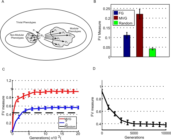
Figure 9. Dynamics of facilitated variation.

(A) Schematic presentation of a phenotypic neighborhood with high facilitated variation. Outer ellipse is the phenotypic space, inner ellipses stand for non-trivial Boolean functions that are within (right ellipse), or without the MVG modularity language (left ellipse), P₀ is the wild-type phenotype and P_1–10 are neighboring phenotypes. The thickness of the arrow represents the probability of the wild-type to generate P_i with one genetic mutation. Length of an edge represents the distance of the phenotypic ‘jump’. High FV corresponds to many long and thick arrows towards the right ellipse. (B) Facilitated variation measure (mean±SE) in RNA model of MVG, FG and a random class of inverse-fold genomes (genomes generated by an algorithm to yield a desired fold) [36] with G1 structure. Data are from 30 simulations in the case of FG and MVG and 200 random genomes. (C) Facilitated variation measure (mean±SE) as a function of generations in logic circuits evolution. Goals were: G1 = (x XOR y) OR (w XOR z), G2 = (x XOR y) AND (w XOR z). For MVG, data are for generations where the goal was G1. Data are from 40 simulations in each case. The random class (dashed line) includes circuits which achieve the goal but were generated by an optimization algorithm rather than by an evolutionary process (see Text S1 section 3.1). (D) Facilitated variation rapidly decays when goal becomes constant over time. Each simulation started from end-of MVG evolution population that had perfect fitness for the goal G1.At the generation marked zero, the population was placed under a FG evolution with the same goal G1, with a selection pressure for minimizing the number of gates [33] (fitness reduction of 0.2/gate for each gate over 10 gates). Mean FV measure (±SE) vs. generations of 500 best-fitness circuits in each population is shown. Statistics are for 30 independent experiments.