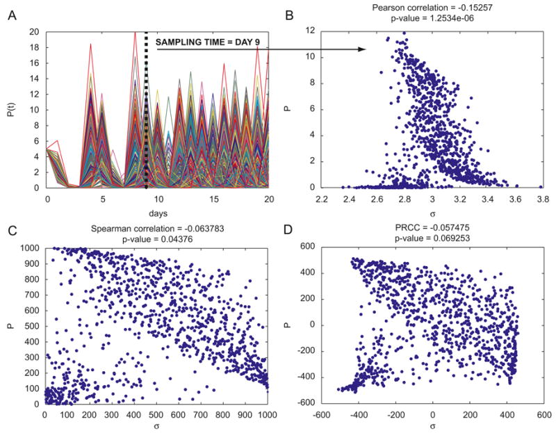
Figure 6.

Panel A: plot of the output (1000 runs) of the Lotka-Volterra model. The y axis represents variable P(t), x axis represents time (days). Panel B: scatter plot (linear scale) of parameter σ (x axis) and the “slice” of the output of Panel A at time=9 (rPearson =-0.15257, p<0.001). Panel C: linear-linear plot of the rank-transformed data of Panel B (rSpearman =-0.0638, p>0.04, where rSpearman is the rPearson coefficient calculated on the data of Panel C.). Panel D: linear-linear plot of the residuals of the linear regressions of the parameter σ versus all the other parameters of the model (x-axis) and the residuals of the linear regression of the output versus parameter σ (y-axis) (PRCC =-0.0575, p>0.06). PRCC is the Pearson correlation coefficient calculated on the data of Panel D. Scatter plots of Panel B, C and D remains qualitatively invariant for different LHS simulations. The input parameter (and its rank-transformed values) shown on the x-axis is σ, although all four parameters are varied simultaneously.
