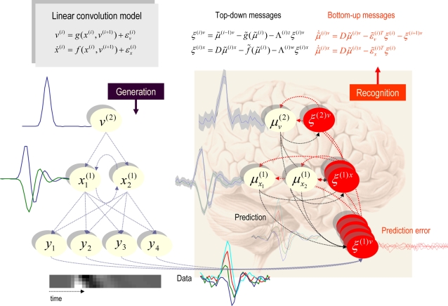
Figure 5. This schematic shows the linear convolution model used in the subsequent figure in terms of a directed Bayesian graph.

In this model, a simple Gaussian ‘bump’ function acts as a cause to perturb two coupled hidden states. Their dynamics are then projected to four response variables, whose time-courses are cartooned on the left. This figure also summarises the architecture of the implicit inversion scheme (right), in which precision-weighted prediction errors drive the conditional modes to optimise variational action. Critically, the prediction errors propagate their effects up the hierarchy (c.f., Bayesian belief propagation or message passing), whereas the predictions are passed down the hierarchy. This sort of scheme can be implemented easily in neural networks (see last section and [5] for a neurobiological treatment). This generative model uses a single cause v ⁽¹⁾, two dynamic states and four outputs y ₁,…,y ₄. The lines denote the dependencies of the variables on each other, summarised by the equations (in this example both the equations were simple linear mappings). This is effectively a linear convolution model, mapping one cause to four outputs, which form the inputs to the recognition model (solid arrow). The inputs to the four data or sensory channels are also shown as an image in the insert.