Figure 1.

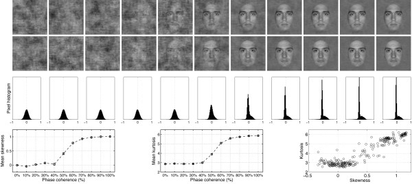
Examples of stimuli used in Experiment 1. The first two rows show the 22 stimuli presented to one observer during the first block of the experiment. The observer discriminated the same two faces during the whole experiment. The noise level varied from 100% (left side; 0% phase coherence) to 0% (right side; 100% phase coherence). Note that at each level of phase coherence the structure of the noise that was mixed with the original image was different, so that the task could not be performed based on the spatial characteristics of the noise. Histograms in the third row show the distribution of pixel contrasts averaged across all stimuli seen by this observer at each level of phase coherence. Starting with a Gaussian distribution (left), the pixel histograms become increasingly skewed and kurtotic with increasing phase coherence (right – the y-axes on the histograms are all the same). This relationship is depicted in the last row, showing the mean skewness (left), and mean kurtosis (middle), as a function of phase coherence. The error bars correspond to 95% confidence interval computed using a bootstrap percentile technique (1000 resamples). In the bottom right end graph, kurtosis for each image (each circle) is expressed as a function of skewness. Although the two statistical descriptors are correlated, the relationship is not linear. As demonstrated below, EEG amplitude is more sensitive to the kurtosis of the image than its skewness.