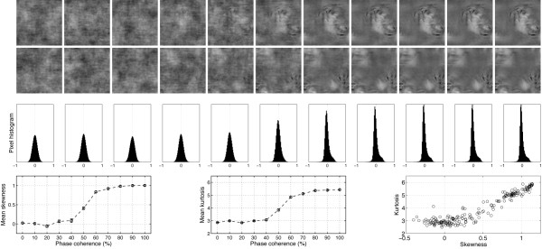
Figure 13.

Examples of stimuli used in Experiment 3. The first two rows show the 22 stimuli presented to one observer during the first block of the experiment. The observer discriminated the same two wavelet textures during the whole experiment. The noise level varied from 100% (left side; 0% phase coherence) to 0% (right side; 100% phase coherence). Histograms in the third row show the distribution of pixel contrasts averaged across the entire set of stimuli seen by this observer at each level of phase coherence, from 0% (left) to 100% (right). Similarly to what was observed for faces in Experiment 1, and contrary to the pink noise textures used in Experiment 2, the pixel histograms showed a non-linear transition from a Gaussian distribution to a skewed and kurtotic distribution with increasing levels of phase coherence. This progression is depicted in the last row, showing the mean skewness (left), and mean kurtosis (middle), as a function of phase coherence. The error bars correspond to 95% confidence interval computed using a bootstrap percentile technique (1000 resamples). In the bottom right end graph, kurtosis for each image (each circle) is expressed as a function of skewness. Similarly to face stimuli, the two statistical descriptors are non-linearly related to one another.