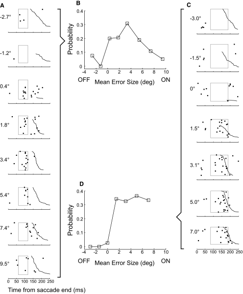
FIG. 8.

Examples of the sensitivity of CS occurrence with error size. A and C: data from units shown in Fig. 3, A and B, respectively. Numbers to the left of each column indicate the mean error size for the trials included in that data set; positive errors are in the preferred direction; negative errors in the opposite direction. As with similar data for direction tuning, trials are aligned on the end of the primary saccade (t = 0) and ordered from top to bottom according to increasing latency of the corrective saccade (jagged black curve). For small error amplitudes around 0, there often was no corrective saccade; as before, those trials were placed at the top of the raster. The rectangles represent MI windows determined from directional tuning data on the same unit. B and D: plots of probability of CS occurrence (within the MI window) against mean error amplitude for the units in A and C, respectively.