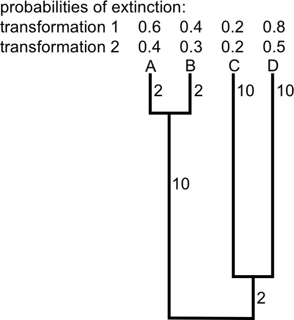
Figure 1. Changing EDGE and HEDGE scores.

EDGE_i = ln(ED_i*Prob(extinction)_i), where ED_i is the sum of edge lengths from the root of the tree to i, each edge length divided by the size of the clade the edge subtends. In figure 1, ED_A = ED_B = 10/2+2/1 = 7, and ED_C = ED_D = 2/2+10/1 = 11. Each species is in a different category of extinction risk (in the rank order of imperilment D,A,B,C ), and these categories have been transformed to prob(extinction) under two scenarios: in the first (power) transformation of extinction categories (Transformation 1), the rank order under EDGE is D (2.2), A (1.4), B(1.0) and C(0.8). With the second (linear) transformation (Transformation 2), C and B switch ranks: D(1.7), A(1.0), C(0.8), and B(0.7). HEDGE_i is also a product of two terms: the expected phylogenetic contribution of a species i given prob(extinction) of all other species, and prob(extinction)_i. However, HEDGE can also be formulated as the change in the total expected PD [28] from the status quo to the expected PD if one sets the prob(extinction)_i = 0, ie. if species i is preserved [15]. The expected PD of a tree can be calculated as the sum of edge lengths, each weighted by its probability of persistence [8]. For example, the expected PD under transformation 1 is 2*0.4+2*0.6+10*(1−0.6*0.4)+0.2*10+0.8*10+(1−0.2*0.8)*2 = 21.3; if we save C, it becomes 2*0.6+2*0.4+10*(1−0.6*0.4)+1*10+0.2*10+(1−0*0.8)*2 = 23.6, and HEDGE_C = 23.6−21.3 = 2.3. The ranked HEDGE list for the species in Figure 1 under transformation 1 is D(8.32), A(3.6), B(3.2), C(2.3). Under transformation 2, the ranked list becomes quite different, with C moving from last to second place: D(5.2), C(2.2), A(2.0), B(1.8).