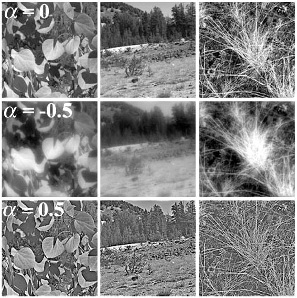
Figure 1.
Examples of the natural images used for tests of blur adaptation. α denotes the slope. The top row presents original images before filtering (α = 0). The middle row presents the same images after filtering with attenuating high and amplified low spatial frequencies (α =−.5). The bottom row presents the images after filtering with amplified high and attenuated low spatial frequencies (α = .5).

