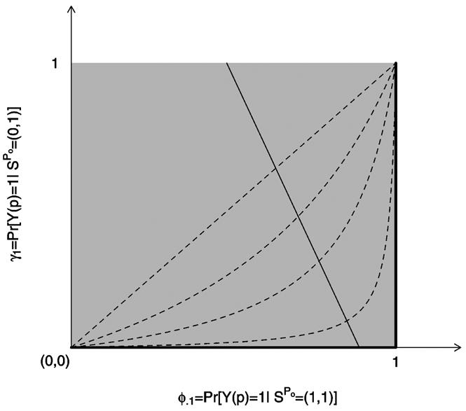
Figure 1.

Graphical Depiction of Selection Bias Models Described in Section 4. The four dotted curves depict the log odds ratio selection model for β = 0, 1, 2, 4. The β = 0 model is equivalent to the no selection model. The thick black lines on the edge of the unit square correspond to the upper-bound selection model. The solid thin line with negative slope represents an example of a family of joint distribution functions of (Z, S(v), S(p), Y(v), Y(p)) for which all combinations of parameters (ϕ.1, γ1) on this line give rise to the same distribution of the observable random variables (Z, Sobs,Yobs). Each selection model identifies exactly one pair of parameters (ϕ.1, γ1) from this family, rendering VEI = 1 − ϕ1./ϕ.1 identifiable.
