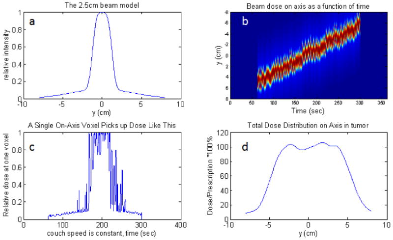
Fig. 8.

Irregular motion with full range sampling in each parameter, 1cm peak to peak amplitude on axis with a 2.5cm beam and all leaves open. The upper-left plot, a, is the beam model. The upper-right,b, is the dose(y,t) function. If one chooses a particular voxel, and plot its dose(t), then the lower left, c, plot is obtained. If one time-integrates the dose for each position, then the dose profile is obtained: lower-right plot, d.
