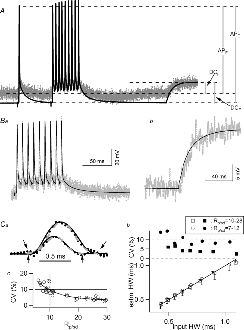
Figure 3. Calibration of fluorescence signals measured in presynaptic terminals.

A, F traces recorded from the cluster of terminals circled in Fig. 2A. The E trace was recorded simultaneously. Action potentials, a single one followed by a train fired at 100 Hz, were initiated during a hyperpolarizing current step. Termination of the current step led to the passive rise near the end of the traces. The two traces are aligned in time but the Y-axes are scaled for the convenience of illustrating various components of measurement. AP_E and AP_F represent the amplitudes of action potential recorded with E and F traces, respectively. DC_E and DC_F represent subthreshold responses arising from termination of a hyperpolarizing current step. Ba, superimposed E and F traces obtained during the 100 Hz train shown in A. The F trace has been scaled to provide the best fit to the E trace, with a scaling constant of 3333. The best fit was determined visually such that the peaks of action potentials, baseline and the depolarizing after-potential all overlap. Bb, superimposed E and F traces obtained during the subthreshold response. The F trace, with a scaling constant of 6863, has been binomially smoothed, 100 points, to better illustrate signals with smaller amplitude. Both E and F traces were averaged from 25 traces. Ca, action potential-like LED transients were used to assess the reliability of action potential half-width estimates. Two examples of LED transients (dotted lines), with signal-to-noise ratios of 20 and 12, respectively, are superimposable with the input LED emission recorded with minimal noise (continuous lines). (See text for details on the generation of these traces and the definition of signal-to-noise ratio (R_p/sd)). Also shown are the Gaussian fits to the LED transients (dashed grey lines). Downward (upward) arrows mark the time window of the Gaussian fit to the LED transient with an R_p/sd value of 20 (12). Cb, lower panel: half-widths recovered from Gaussian fits plotted against half-widths of the corresponding input LED emission. Each data point, with standard deviation for its error bar, is the average of 10 trials and each trial is an average of 20 traces. Recovered half-widths match those of the input transients perfectly. The coefficient of variation calculated from each point is displayed on the upper panel. The squares represent LED transients with an R_p/sd value between 10 and 28, whereas the circles were calculated from a separate series with an R_p/sd range of 7–12. Cc, correlation between the coefficient of variation of recovered half-widths and the R_p/sd of the LED transients from which half-width estimates were calculated. The vertical and horizontal lines highlight that in order to keep the coefficients of variation of the estimated half-width under 10%, the R_p/sd value should be at least 10.