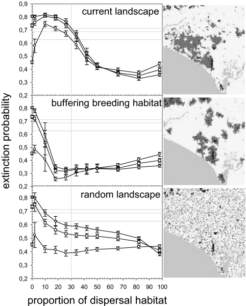
Fig. 3.
Extinction probability in 100 years for landscapes with different levels of matrix heterogeneity. We considered the current landscape configuration (Top), a distribution of dispersal habitat buffering breeding habitat (Middle), and a random distribution of dispersal habitat (Bottom). In all cases, we only changed the proportion of dispersal/open habitats. The three maps show an example for each landscape configuration (dark gray represents breeding habitat, light gray barrier—the lower left corner is the Atlantic ocean—, intermediate gray dispersal habitat and white open habitat). We used three scenarios depending on the increase of risk of mortality during dispersal when individuals move in more fragmented areas (circles, no effect ρ = 0; squares, field estimate of the risk increase ρ = 5.8; triangles, ρ = 10; see The Movement Submodel and Model Parameterization in SI Appendix). In the three cases, the baseline mortality during dispersal was adjusted. The vertical gray line marks the proportion of dispersal habitat present in the current real landscape. Symbols are the average extinction probabilities for five landscape replicates (±SD). The three horizontal gray lines represent the extinction probabilities in the current landscape for the three risk scenarios.

