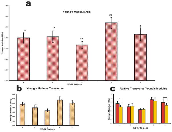
Figure 8.
(a) Plot showing the trend for Axial Young’s modulus using an established Poisson’s Ratio in the Hertz model equation. * denotes regions significantly different from region D, # denotes regions significantly different from region C, and ** or ## denotes an alpha level of below 0.01. (b) Plot showing trend for Transverse Young’s modulus using the indentation ratio in the Hertz model equations. * denotes regions significantly different from region D, # denotes regions significantly different from region C, % denotes regions significantly different from E and ** or ## denotes and alpha level of below 0.01. (c) Plot showing the trend between axial and transverse scans * denotes difference between directions, ~ denotes region reasonably close to 0.05.

