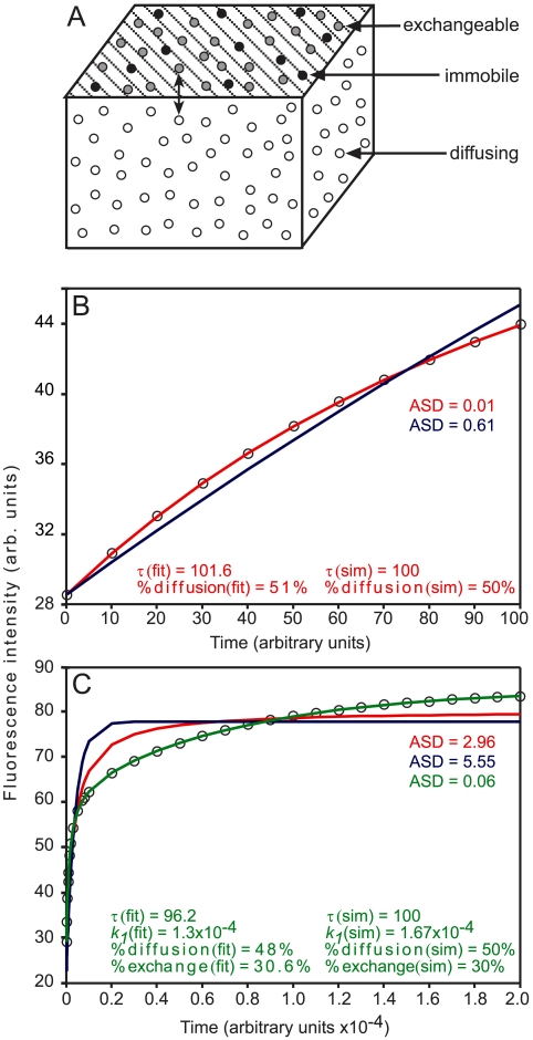
Figure 3. 3D simulation of plaque protein dynamics and fitting to analytical expressions for different FRAP mechanisms.

(A) Schematic representation of the model for plaque protein dynamics. The particles (molecules of FA plaque proteins) undergo fast 3D diffusion (random walk) in a cubic volume, and reversible binding to one of the volume boundaries (stripes). The bound molecules are assumed to be laterally immobile, to mimic FAs on the experimental timescale. A fraction of the bound molecules can, however, undergo exchange (slow, relative to the diffusion) with the free molecules. (B–C) FRAP simulations and fittings to different mechanisms. A CTRW algorithm [31], [32] was used to simulate FRAP experiments in a system modeled after paxillin and vinculin dynamics in FAs. The simulation parameters were chosen to resemble those of the FRAP experiments (Figures 1 and 2). Since the R_f values of both proteins at FAs on the short timescale were around 0.50 (Figure 1D), 50% of the particles were denoted as undergoing 3D diffusion. Based on the increase in R_f to ∼0.80 on the longer timescale (Figure 1E), the remaining 50% of the particles were divided, with 30% undergoing exchange, and 20% immobile. τ for diffusion (τ_D) was introduced (in arbitrary units; au) as 100. To simulate a ∼60-fold slower exchange rate (see Figure 4), we introduced 1/b = τ_D×60 = 100×60 au, i.e., b = 1.67×10⁻⁴, where b represents the dissociation rate constant. (B) Short timescale. Under such conditions, the contribution of slow exchange was negligible, and it was sufficient to consider only the 3D diffusion. This was evident from the excellent fit of the data to the analytical expression for FRAP by lateral diffusion [24] (Eq. 14; red line). Fitting to exchange (Eq. 17; blue line) was much worse (Average Squared Deviation - ASD - values are shown). Fitting to two subpopulations (Eq. 18) did not improve the fit (data not shown). The parameters derived by fitting to lateral diffusion were similar to those introduced in the simulation [panel (B)]. Thus, the analytical expression for lateral diffusion [24] (Eq. 14) could be used to fit 3D diffusion. (C) Long timescale. At this timescale, the contribution of exchange becomes significant. The situation could be approximated by two subpopulations, one recovering by fast diffusion, and one by slow exchange (Eq. 18). Diffusion (red) or exchange (blue) alone did not fit. However, the analytical expression for two populations (Eq. 18; green) yielded a good fit. The fitted parameters were in agreement with those introduced in the simulation [Panel (C)].