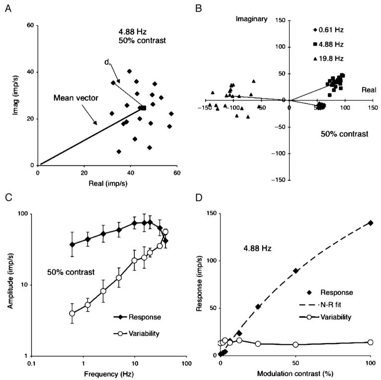
Figure 1.

Basics of response analysis. (A) Each point represents real and imaginary components from the Fourier analysis of one cycle of response of a +L−M parvocellular (PC) cell to chromatic modulation at 4.88 Hz, 50% contrast. The square shows the mean response and the mean vector is drawn in. d_i is the distance between each point and mean and is used to calculate noise as described in the text.(B) Responses of a +L−M PC cells at three temporal frequencies; 50% modulation. Individual cycles and mean vectors are shown. The scatter increases substantially with temporal frequency although length of the response vector increases only moderately. The mean vector rotates due to response latency. (C) Response amplitude (signal) and variability (noise) as a function of temporal frequency. Mean of five PC cells, both +M−L and +L−M cells combined, 50% modulation. Variability increases more steeply with temporal frequency than does amplitude, resulting in a decrease in signal-to-noise ratio. (D) Response amplitude and variability for a +L−M PC cell as a function of contrast at 4.88 Hz. Response amplitude increases with contrast but variability remains constant. Responses have been fitted by a Naka–Rushton function.