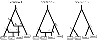
Fig. 1.

First example: the three evolutionary scenarios. The dataset used as an example has been simulated according to scenario 1 (left). The parameter values were the following: all populations had an effective (diploid) size of 1000, the times of successive events (backward in time) were t₁ = 10, t₂ = 500, t₃ = 10 000, t₄ = 20 000 and t₅ = 200 000, the two admixture rates were r₁ = 0.6 and r₂ = 0.4. Scenario 1 includes six populations, the four that have been sampled and two left parental populations in the admixture events. Scenario 2 and 3 include 5 and 4 populations, respectively. Samples 3 and 4 have been collected 2 and 4 generations earlier than the first two samples, hence their slightly upward locations on the graphs. Time is not at scale.