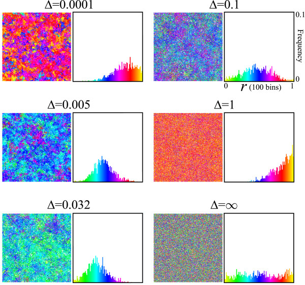
Figure 2.
Snapshots of simulations & population distribution of r. The right panels in each pair show a population distribution of r at a given time-step of simulations [where r = kDM/(kDM + kDP)]. Population distributions of r were observed after the system reached equilibrium. The abscissa is r in the range of [0,1] with 100 bins. The coordinate is the frequency of individuals (P or M or D) in the range of [0,0.1] (the sum of frequencies is normalized to 1). The left panels show the spatial distribution of individuals colored by value of r. Colors indicate values of r at the same time step as that of the population distribution of r (right panels). The values of the parameters are as follows: kSP = kSM = kDP + kDM = 1 (replication rates); d = 0.01 (decay rate); μ = 0.01 (mutation rate); δr = 0.1 (mutation step).

