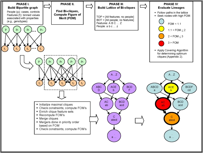
Figure 1. Overview of the Bi-clique-Finding Algorithm.

Step 1 involves the construction of bipartite graph to identify all relationships between nodes (Figure 1, Phase I). In Step 2, the algorithm undertakes maximal bi-clique formation by exhaustively searching the entire space of all genotype combinations to identify an initial set of maximal bi-cliques (Figure 1, Phase II). In the third step, a Figure of merit (FOM) is generated to prioritize “interesting” bi-cliques (Figure 1, Phase II). The FOM can be any measure inherent to the data. Here, we consider values of features (e.g., genotypes) in a 2×2 contingency Table with affected cases and unaffected controls contingent on exposure (e.g., genotype). In the fourth step, a “lattice” is built by connecting each pair of bi-cliques to their least upper bound and their greatest lower bound using principles of set union and intersection. (Figure 1, Phase III). In the fifth step, the bi-cliques of greatest interest are identified using a parsimony principle by which “optimal” bi-cliques should contain the most parsimonious set of features, and the addition of more features does not substantially improve the FOM. To achieve this, we employ the set covering approach[33] (Appendix S1).