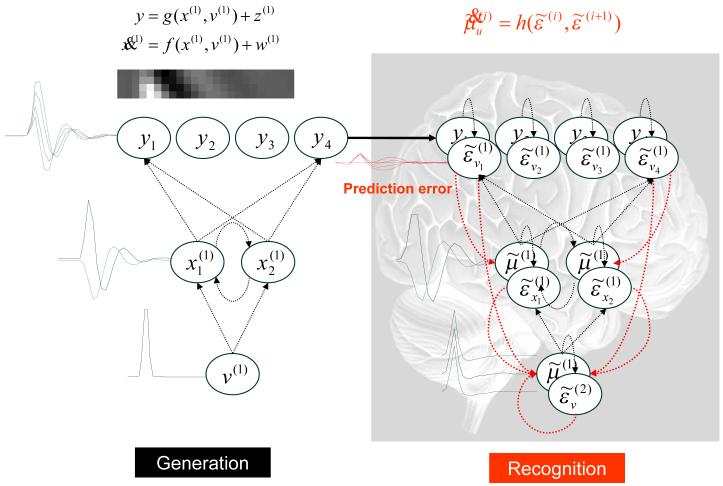
Figure 4.

Diagram showing the generative model (left) and corresponding recognition; i.e., neuronal model (right) used in the simulations. Left panel: this is the generative model using a single cause v⁽¹⁾, two dynamic states $x_1^{\left(1\right)},x_2^{\left(1\right)}$ and four outputs y₁,K, y₄. The lines denote the dependencies of the variables on each other, summarised by the equation on top (in this example both the equations were simple linear mappings). This is effectively a linear convolution model, mapping one cause to four outputs, which form the inputs to the recognition model (solid arrow). The architecture of the corresponding recognition model is shown on the right. This has a corresponding architecture, but here the prediction error units, ${\tilde{\epsilon }}_u^{\left(i\right)}$, provide feedback. The combination of forward (red lines) and backward influences (black lines) enables recurrent dynamics that self-organise (according to the recognition equation; ${\tilde{\mu }}_u^{\left(i\right)}=h({\tilde{\epsilon }}^{\left(i\right)},{\tilde{\epsilon }}^{(i+1)}))$ to suppress and hopefully eliminate prediction error, at which point the inferred causes and real causes should correspond.