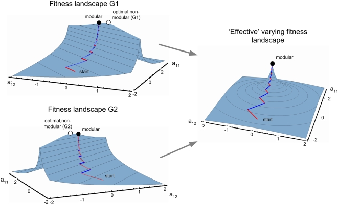
Figure 6. Fitness landscape illustration (a two dimensional system).

Goals G₁, G₂ are as described in Figures 4,5. The fitness landscapes are presented as a projection on the hyper-surfaces (a₂₁, a₂₂) of the optimal solution [i.e. (0.5,0.5) for G₁, (−0.5, 0.5) for G₂, and (0, 1) for MVG]. A typical trajectory is shown under MVG, switching between G₁ and G₂ as described in Figure 5. red/blue: dynamics under fitness landscape G₁ and G₂ respectively. Fitness is presented in log scale. Full/empty circle represents the modular/non-modular solutions. The fitness landscapes under constant goals are characterized by a single ridge (with slow dynamics as shown in Figures 4B and 4C). Under MVG the effective fitness landscape forms a steep peak where a solution that solves both goals resides (the modular solution). To ease comprehension, we chose a different viewing angle from the one of Figures 4,5. Switching time is E = 100/r.